These is a summary of the functionalities present in slabbe-0.2.spkg optional Sage package. It works on version 6.8 of Sage but will work best with sage-6.10 (it is using the new code for cartesian_product merged the the betas of sage-6.10). It contains 7 new modules:
- finite_word.py
- language.py
- lyapunov.py
- matrix_cocycle.py
- mult_cont_frac.pyx
- ranking_scale.py
- tikz_picture.py
Cheat Sheets
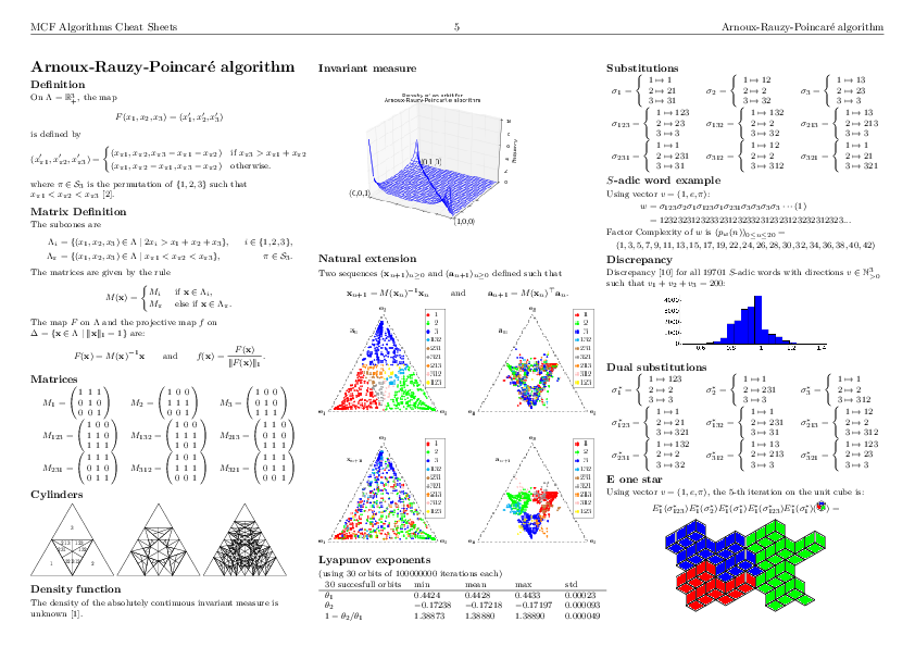
The best way to have a quick look at what can be computed with the optional Sage package slabbe-0.2.spkg is to look at the 3-dimensional Continued Fraction Algorithms Cheat Sheets available on the arXiv since today. It gathers a handful of informations on different 3-dimensional Continued Fraction Algorithms including well-known and old ones (Poincaré, Brun, Selmer, Fully Subtractive) and new ones (Arnoux-Rauzy-Poincaré, Reverse, Cassaigne).
Installation
sage -i http://www.slabbe.org/Sage/slabbe-0.2.spkg    # on sage 6.8
sage -p http://www.slabbe.org/Sage/slabbe-0.2.spkg    # on sage 6.9 or beyond
Examples
Computing the orbit of Brun algorithm on some input in \(\mathbb{R}^3_+\) including dual coordinates:
sage:fromslabbe.mult_cont_fracimportBrunsage:algo=Brun()sage:algo.cone_orbit_list((100,87,15),4)[(13.0,87.0,15.0,1.0,2.0,1.0,321),(13.0,72.0,15.0,1.0,2.0,3.0,132),(13.0,57.0,15.0,1.0,2.0,5.0,132),(13.0,42.0,15.0,1.0,2.0,7.0,132)]
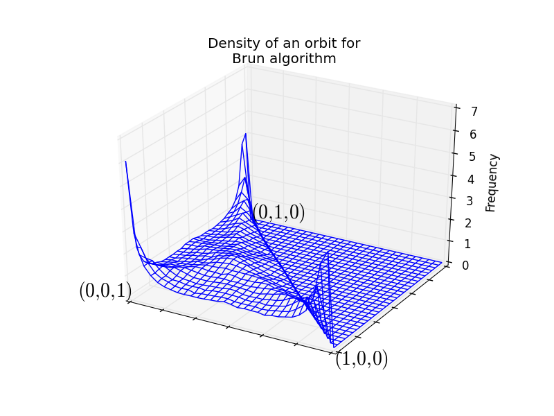
Computing the invariant measure:
sage:fig=algo.invariant_measure_wireframe_plot(n_iterations=10^6,ndivs=30)sage:fig.savefig('a.png')
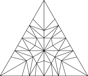
Drawing the cylinders:
sage:cocycle=algo.matrix_cocycle()sage:t=cocycle.tikz_n_cylinders(3,scale=3)sage:t.png()
Computing the Lyapunov exponents of the 3-dimensional Brun algorithm:
sage:fromslabbe.lyapunovimportlyapunov_tablesage:lyapunov_table(algo,n_orbits=30,n_iterations=10^7)30succesfullorbitsminmeanmaxstd+-----------------------+---------+---------+---------+---------+$\theta_1$0.30260.30450.30510.00046$\theta_2$-0.1125-0.1122-0.11150.00020$1-\theta_2/\theta_1$1.36801.36841.36890.00024
Dealing with tikzpictures
Since I create lots of tikzpictures in my code and also because I was unhappy at how the view command of Sage handles them (a tikzpicture is not a math expression to put inside dollar signs), I decided to create a class for tikzpictures. I think this module could be usefull in Sage so I will propose its inclusion soon.
I am using the standalone document class which allows some configurations like the border:
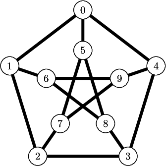
sage:fromslabbeimportTikzPicturesage:g=graphs.PetersenGraph()sage:s=latex(g)sage:t=TikzPicture(s,standalone_configs=["border=4mm"],packages=['tkz-graph'])
The repr method does not print all of the string since it is often very long. Though it shows how many lines are not printed:
sage:t
\documentclass[tikz]{standalone}
\standaloneconfig{border=4mm}
\usepackage{tkz-graph}
\begin{document}
\begin{tikzpicture}%
\useasboundingbox(0,0)rectangle(5.0cm,5.0cm);%
\definecolor{cv0}{rgb}{0.0,0.0,0.0}......68linesnotprinted(3748charactersintotal)......
\Edge[lw=0.1cm,style={color=cv6v8,},](v6)(v8)
\Edge[lw=0.1cm,style={color=cv6v9,},](v6)(v9)
\Edge[lw=0.1cm,style={color=cv7v9,},](v7)(v9)%
\end{tikzpicture}
\end{document}
There is a method to generates a pdf and another for generating a png. Both opens the file in a viewer by default unless view=False:
sage:pathtofile=t.png(density=60,view=False)sage:pathtofile=t.pdf()
Compare this with the output of view(s, tightpage=True) which does not allow to control the border and also creates a second empty page on some operating system (osx, only one page on ubuntu):
sage:view(s,tightpage=True)
One can also provide the filename where to save the file in which case the file is not open in a viewer:
sage:_=t.pdf('petersen_graph.pdf')
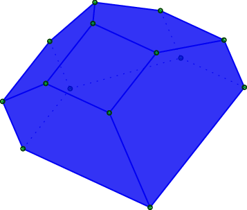
Another example with polyhedron code taken from this Sage thematic tutorial Draw polytopes in LateX using TikZ:
sage:V=[[1,0,1],[1,0,0],[1,1,0],[0,0,-1],[0,1,0],[-1,0,0],[0,1,1],[0,0,1],[0,-1,0]]sage:P=Polyhedron(vertices=V).polar()sage:s=P.projection().tikz([674,108,-731],112)sage:t=TikzPicture(s)sage:t
\documentclass[tikz]{standalone}
\begin{document}
\begin{tikzpicture}%[x={(0.249656cm,-0.577639cm)},y={(0.777700cm,-0.358578cm)},z={(-0.576936cm,-0.733318cm)},scale=2.000000,......80linesnotprinted(4889charactersintotal)......
\node[vertex]at(1.00000,1.00000,-1.00000){};
\node[vertex]at(1.00000,1.00000,1.00000){};%%%%
\end{tikzpicture}
\end{document}sage:_=t.pdf()