We are the SageMathCloud developers!
This is just a test and we love math:
$\Phi(x) = \frac{1}{\sqrt{2 \pi}} \int_{-\infty}^x e^{-\xi^2/2}\; d\xi$
Expect more soon!
We are the SageMathCloud developers!
This is just a test and we love math:
$\Phi(x) = \frac{1}{\sqrt{2 \pi}} \int_{-\infty}^x e^{-\xi^2/2}\; d\xi$
Expect more soon!
By default, running a cell in a Sage worksheet causes the input to be run as Sage commands, with output from Sage written to the output of the cell. Mode commands in a Sage worksheet cause the input to be run through some other process to create cell output. For example,
%md at the start of a cell causes cell input to be rendered as markdown in the cell output.%r causes cell input to be treated as statements in the R language, with corresponding output.%HTML causes cell input to be treated as HTML, rendered as the output.There are many built-in modes (e.g. Cython, GAP, Pari, R, Python, Markdown, HTML, etc…)
Note: If it is not the default mode of your *.sagews worksheet, a mode command must be the first line of a cell. In other words, make sure the command %md, %r, or %HTML is the first line of a cell.
Alternatively, you can make any mode the default for all cells in the worksheet using %default_mode <some_mode>. Then all cells will be using that chosen mode. If you choose this approach, you may still explicitly use %sage for cells you want processed by the Sage interpreter (or %foo to explicitly switch to any non-default mode).
There is an entire section of the FAQ page SageMathCloud Worksheet (and User Interface) Help dedicated to questions about the built-in modes. It had 10 questions-and-answers in it as of July 28, 2016.
You can view available built-in modes by selecting Help > Mode commands in the Sage toolbar while cursor is in a sage cell. That will
insert the line print('\n'.join(modes())) into the current cell.
Custom mode commands are modes defined by the user. Like any mode command, a custom mode command processes the input section of a cell and writes the output. As stated in the help for modes,
Create your own mode command by defining a function that takes a string as input and outputs a string. (Yes, it is that simple.)
Custom mode commands can be used to - render or compile cell input into cell output - send commands to other processes and show the results
Here are some examples:
Define the mode in a sage cell, as follows:
importpandasaspdfromStringIOimportStringIOdefcsv_table(str):print(pd.read_csv(StringIO((str)),index_col=0))Input:
%csv_table
Sample,start,middle,end
A,2,5,51
B,6,8,11
C,7,22,41
Output:
        start  middle  end
Sample
A           2       5   51
B           6       8   11
C           7      22   41
NOTE: Sage’s show command is also aware of Pandas tables,
so if you instead define
defcsv_table(str):show(pd.read_csv(StringIO((str)),index_col=0))then %csv_table will produce nice HTML output.
Define the mode:
importjsonimportyamldefj2y(str):print(yaml.safe_dump(json.loads(str)))Input:
%j2y{"foo":"bar","baz":["xyzzy","plugh"]}Output:
baz:[xyzzy,plugh]foo:barIn this example, each input line is a number with units, possibly followed by target units. If target units are not specified, SI units are the target. This example uses the Sage Units of Measurement package.
Define the mode:
defconvert_units(str):forlineinstr.split('\n'):if'units'inline:lval=eval(line)ifisinstance(lval,tuple):print(lval[0].convert(lval[1]))else:print(lval.convert())Input:
%convert_units# pounds to kilograms175.0*units.mass.pound# miles to kilometers3.0*units.length.mile,units.length.kilometer# an adult doing moderate exercise might burn 200 kcal per hour# convert to watts200.0*units.energy.calorie*units.si_prefixes.kilo/units.time.hour,units.power.wattOutput:
79.37866475*kilogram4.828032*kilometer232.6*wattThis example uses Biopython, which is already installed on SageMathCloud.
Define the mode:
fromBio.SeqimportSeqdefrevcomp(str):s=Seq(str)print(s.reverse_complement())Input:
%revcompATGCGCTCCGACACTTTOutput:
AAAGTGTCGGAGCGCATSuppose you want several bash processes with different working directories or environment variables controlled from the same worksheet. You can use the built-in jupyter command to create several custom modes.
More information on “the sage-jupyter bridge” is available at Sage Jupyter. Code creating a mode for anaconda3 is available by selecting Modes > Jupyter bridge. You can view available Jupyter kernels by selecting Help > Jupyter kernels in the Sage toolbar while cursor is in a sage cell. That will
insert the line print(jupyter.available_kernels()) into the current cell.
Define the modes:
sh1=jupyter("bash")sh2=jupyter("bash")Cell 1:
%sh1# show PID of current sh processecho$BASHPID--output--23723Cell 2:
%sh2echo$BASHPID--output--23727Cell 3:
%sh1echo$BASHPID--output--23723In this example, any cell in the custom mode consists of shell commands to be run on a remote server. The same session is used for all cells in the given mode.
Notes: - The SageMathCloud project must have Internet access. This is an upgrade, only available to users with a paid subscription. (See also “Why Should I Purchase a Subscription?”.) - Configure ssh public and private keys with empty passphrase. - Set host and user for the remote connection. - You may want to set IdentityFile in your ~/.ssh/config file.
Define the mode:
%sagefrompexpectimportpxsshfromansi2htmlimportAnsi2HTMLConverterconv=Ansi2HTMLConverter(inline=True,linkify=True)s=pxssh.pxssh(echo=False)host='myhost.mydomain.org'user='joe'ifs.login(host,user):defsshexec(code):forlineincode.split('\n'):s.sendline(line)s.prompt()h=s.beforeh=conv.convert(h,full=False)h='<pre style="font-family:monospace;">'+h+'\n</pre>'salvus.html(h)print'sshexec defined; logout with s.logout()'else:print'sshexec setup failed'Input:
%sshexeclscd/tmpOutput:
...lslisting,showingcolor-lsoutputifavailable...Input in second cell, showing that working directory is retained
%sshexecpwdThe following function takes whatever the cell input is, executes the code in FriCAS, performs some simple substitutions on the FriCAS output and then displays it using Markdown:
Define the mode:
%sagedeffricas_tex(s):importret=fricas.eval(s)t=re.compile(r'\r').sub('',t)# mathml overbart=re.compile(r'¯').sub('‾',t,count=0)# cleanup FriCAS LaTeXt=re.compile(r'\\leqno\(.*\)\n').sub('',t)t=re.compile(r'\\sb ').sub('_',t,count=0)t=re.compile(r'\\sp ').sub('^',t,count=0)md(t,hide=False)With this mode, FriCAS can generate output that is (almost) compatible with Markdown format.
For example you can use this new mode in a cell with the following input:
%fricas_tex)setoutputalgebraoff)setoutputmathmlon)setoutputtexonsqrt(2)/2+1Output: This will evaluate ‘sqrt(2)/2+1’ and display the result in both LaTeX format and MathML formats (in a MathML capable browser).
Note: The current version of Sage (6.6 and earlier) requires a patch to correct a bug in the fricas/axiom interface.
For a quick reminder, sample code is available for opening an Anaconda3 session. In the Sage worksheet toolbar, select Modes > Jupyter bridge.
Use the jupyter command to launch any installed Jupyter kernel from a Sage worksheet
py3=jupyter("python3")After that, any cell that begins with %py3 will send statements to the Python3 kernel that you just started. If you want to draw graphics, there is no need to call %matplotlib inline.
%py3print(42)importnumpyasnp;importpylabaspltx=np.linspace(0,3*np.pi,500)plt.plot(x,np.sin(x**2))plt.show()You can set the default mode to be your Jupyter kernel for all cells in the worksheet: after putting the following in a cell, click the “restart” button, and you have an anaconda worksheet.
%autoanaconda3=jupyter('anaconda3')%default_modeanaconda3Each call to jupyter() launches its own Jupyter kernel, so you can have more than one instance of the same kernel type in the same worksheet session.
p1=jupyter('python3')p2=jupyter('python3')p1('a = 5')p2('a = 10')p1('print(a)')# prints 5p2('print(a)')# prints 10William scripted status reports, organized several things related to billing, and spent hours working on subtle issues related to sync and file saving. Harald worked on the SMC blog, read emails, and triaged tickets. Hal continued experiments with pytest for smc_sagews, resumed work on sagews issues (note PR823 is ready for review), updated MOOC companion for complex variables, and explored supporting .Rmd files and %Rmd sagews mode. Tim made three pull requests for realtime list of collaborators viewing any file in a project, restoring tabs, and make deletion immediately delete files from disk instead of moving them to the trash, since we have snapshots.
Our Nightly Changelog keeps you updated on small feature changes, bugfixes, and quality of life improvements. For upcoming changes, see our weekly progress report column.
"Google open source guru Chris DiBona says that the web giant continues to ban the lightning-rod AGPL open source license within the company because doing so "saves engineering time" and because most AGPL projects are of no use to the company."This is just the way it is -- it's psychology and culture, so deal with it. In contrast, companies very frequently embrace open source code that is licensed under the Apache or BSD licenses, and they keep such projects alive. The extremely popular PostgreSQL database is licensed under an almost-BSD license. MySQL is freely licensed under the GPL, but there are good reasons why people buy a commercial MySQL license (from Oracle) for MySQL. Like RethinkDB, MongoDB is AGPL licensed, but they are happy to sell a different license to companies.
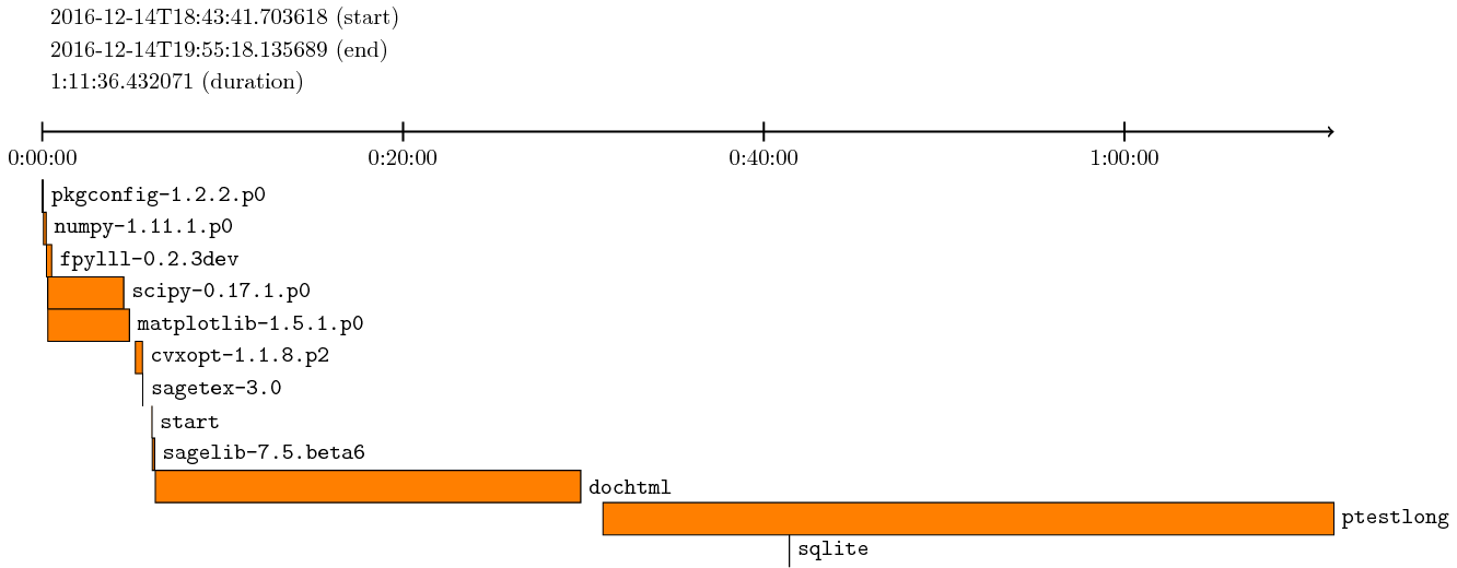
Compiling sage takes a while and does a lot of stuff. Each time I am wondering which components takes so much time and which are fast. I wrote a module in my slabbe version 0.3b2 package available on PyPI to figure this out.
This is after compiling 7.5.beta6 after an upgrade from 7.5.beta4:
sage:fromslabbe.analyze_sage_buildimportdraw_sage_buildsage:draw_sage_build().pdf()
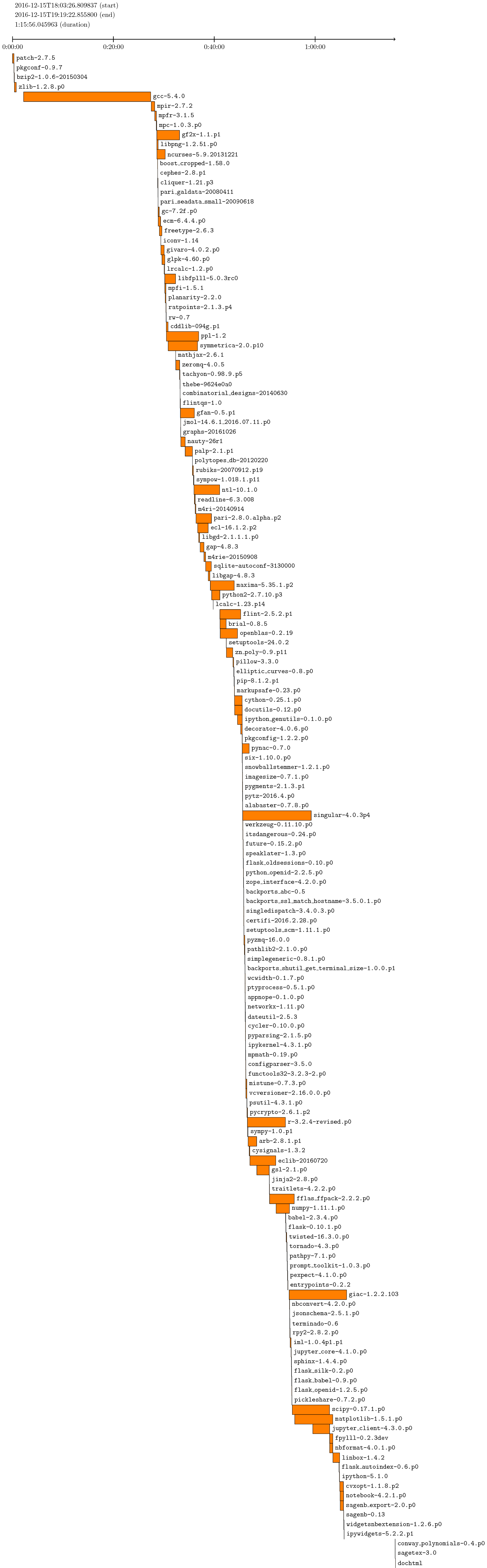
From scratch from a fresh git clone of 7.5.beta6, after running MAKE='make-j4' make ptestlong, I get:
sage:fromslabbe.analyze_sage_buildimportdraw_sage_buildsage:draw_sage_build().pdf()
The picture does not include the start and ptestlong because there was an error compiling the documentation.
By default, draw_sage_build considers all of the logs files in logs/pkgs but options are available to consider only log files created in a given interval of time. See draw_sage_build? for more info.
I’ve been participating in the Kan Extension Seminar II, and this week it’s my turn to post about Jon Beck’s “Distributive Laws” at the n-Category Cafe!
The post uses lots of string diagrams for monads, resulting in pictures like the following:

See you there!
This project seeks to implement several common matroid classes in SageMath, along with algorithms for their display and relevant computations. The graphic matroid class in particular will be implemented with a representative graph with methods for Whitney switching and minor operations. This will be accompanied by improvements to the graph theory library, with methods relevant to matroids enabled to support multigraphs. Other modules for this project include improved plotting of rank 3 matroids to eliminate false colinearities, computation of a matroid's automorphism group using SageMath's group theory libraries, and faster minor testing based on an existing trac ticket.
As a member of the sage-dynamics community, researchers have compiled a wishlist for algorithms and functionality they would like added. I would like to shorten the wish list for us.For my project I will be completing some desired additions to SAGE from the Sage Dynamics Wiki. I will implement Well’s Algorithm, strengthen the numerical precision in cannonical_height, as well as implement reduced_form for higher dimensions.
There are three major things that I would like to implement to improve the functionality of Sage in the area Complex Dynamics. The details of the project are summarized in the following list:
- Complex Dynamics Graphical package: Integrate or implement a complex dynamics software such as Mandel into Sage. This will be done by creating an optional package for Sage. If there is enough demand, the package may become a standard package for Sage at some point.
- Spider Algorithm: The object of the Spider Algorithm is to construct polynomials with assigned combinatorics. For example, we may want to find a polynomial that has a periodic orbit of period 7. The Spider Algorithm provides a way for us to compute this polynomial efficiently. I plan to implement this algorithm into Sage.
- Coercion: If you have a map defined over Q, you should be able to take the image of a point over C (i.e. somewhere you have a well-defined embedding) without having to use the command "change_ring()". Something similar works for polynomials in Sage but it does not work for morphisms/schemes.
This project is aimed at providing linear time implementation for modular decomposition of graphs and digraphs. Modular decomposition is decomposition of graph into modules. A module is a subset of vertices and it is a generalization of connected component in graph. Let us take for example a module X. For any vertex v ∉ X it is either connected or not connected to every vertex of X. Another property of module is that a module can be subset of another module. There are various algorithms which have been published for modular decomposition of graphs. The focus in this project is on linear time complexity algorithms which can be practically implemented. The project further aims to use the modules developed for modular decomposition to implement other functionality like skew partitions. Skew partition is partition of graph into two sets of vertices such that induced graph formed by one set is disconnected and induced graph formed by other set is complement of the first. Modular decomposition is a very important concept in Graph Theory and it has a number of use cases. For instance it has been an important tool for solving optimization and combinatorics problems.
Modular decomposition of (di)graphs is a generalization of the concept of the decomposition of (di)graphs into connected components. Its current implementation in Sage relies on badly broken abandoned C code, and badly needs to be replaced by something that works and is not too slow. However, the only open-source implementations of some of these procedures are either in Java or in Perl, and thus aren't really useful for Sage.
I aim to implement visualizations of several key constructs in cluster algebras and quiver representations. The first is Auslander-Reiten quivers, for at least the A_n and D_n cases. The second is labelled endomorphism quivers and mutations within a cluster category, focusing on the A_n case. The third is posets of down-mutations for the A_n case. These features will be useful not only for research purposes, but also as nice examples to play around with and learn from. Aside from these features, I am interested in implementing features for the Quantum Cluster Algebras project.
Hans Fangohr presented the first prototype of the Python OOMMF interface at the 61st international meeting on magnetism and magnetic materials in New Orleans (US).