Quantcast
Channel: Planet Sage
Viewing all 414 articles
Browse latest View live

Liang Ze: Partitions and Posets

$
0
0

In this post, we generate the Hasse diagram of a set partition.

Partitions of a 4 element set

The following piece of code generates the image above.

Read on for an explanation of the code.

Partitions

A partition of a set $X$ is a collection $p$ of non-empty subsets of $X$ such that $X$ is the disjoint union of these sets.

In SAGE, you can get the set of all partitions of the $N$ element set {$1,2,\dots,N$} using SetPartitions:

Refinements

Each item in the preceding list is a partition of $X$. The elements of each partition are called blocks. At the top of the list, we see the trivial partition consisting of just one block, $X$. At the other end, we see the singleton partition consisting of $|X|$ blocks, where each block contains a single element of $X$. All other partitions of $X$ fall somewhere in-between these two partitions.

We can make this notion of “in-betweenness” precise by defining a relation on the partitions of $X$. We say that $q$ is a refinement of $p$ if each block of $q$ is contained in some block of $p$.

In Sage, you can see the refinements of a partition using the method refinements():

Posets

For a fixed $X$, the set $\mathcal{P}$ of all partitions of $X$ has the structure of a poset given by $q \leq p$ if $q$ is a refinement of $p$.

In Sage, we can construct a Poset by specifying an underlying set $P$ along with a function $f:P\times P \to$ {$\text{True},\text{False}$} where

The resulting poset can be visualized via its Hasse diagram, which is a directed graph with paths from $q \to p$ if $q \leq p$. We can generate a Hasse diagram of a poset using the show() method.

The final piece of code (at the top of the page) combines everything above to produce the Hasse diagram of a set. The function Partition_Poset first generates the set of partitions of an $N$ element set, then converts it to a poset. The function p_label relabels the partitions so that they look prettier. I’ve also tweaked some options in the show() method to make things look nicer.


Liang Ze: The Argument Principle

$
0
0

This post illustrates the Argument Principle.

Let $f$ be a polynomial, and $C$ be (an arc of) a circle of radius $R$ centered at the origin.

The code below generates 2 plots. The first plot shows the domain of $f$. We plot the roots of $f$ together with $C$. Let $n_1$ be the number of roots contained within $C$.

The second plot shows the range of $f$. We plot $f(C)$, along with a marker at the origin. Let $n_2$ be the number of times the curve winds around the origin.

You can verify that $n_1 = n_2$. As you vary the radius $R$, observe how $C$ and $f(C)$ change, and how this affects $n_1$ and $n_2$.

Liang Ze: Lattice of Subgroups

$
0
0

This is the first in a series of posts on visualizing groups via their lattice of subgroups.

Lattice of the dihedral group $D_4$

Displaying the Lattice of Subgroups

One way of getting a better understanding of a group is by considering its subgroups. The lattice of subgroups (more precisely, the Hasse diagram of this lattice) gives us a way to visualize how these subgroups relate to each other and to their parent group. Here’s how to do it in Sage:

(The Sage cells in this post are linked, so things may not work if you don’t execute them in order.)

By default, the vertex labels of the Hasse diagram will be the description of the object that the vertex represents. In our case, something like Subgroup of (Dihedral group of order 8 as a permutation group) generated by [(1,2)(3,4)], which would be way too long to display nicely. Because of this, in the above code, I’ve decided not to label the vertices. I’ve also chosen to make the vertices hexagonal and white.

Relabelling vertices

Without labels, it can be hard to tell what subgroups we’re looking at. We can define new labels for these vertices by defining a dictionary where the keys are the original vertices and their corresponding values are our new labels.

Labelling by generators

One way to tell what the subgroups are is to look at their generators:

This isn’t very pretty, and just knowing the generators doesn’t give us much intuition about the group.

Labelling by cardinalities

Alternatively, we could label the subgroups by their cardinalities:

If you ran the preceding code, you probably encountered an error message. This is because Sage currently requires that vertex labels be injective i.e. distinct vertices must have distinct labels. There’s a quick but slightly ugly fix for this: just pad spaces around the labels to make them all unique:

Labelling by structure description

However, cardinalities still don’t tell me very much about the subgroup. Fortunately, Sage has a method for describing the structure of a small group: H.structure_description() where H is the group in question.

Unfortunately, this method requires the GAP group database, which is not installed with the Sagecell version of Sage. However, the free SageMathCloud service’s installation of Sage does have the group database installed, so you can try the following code there. This code was used to produce the image at the start of this post:

More examples

Try playing around with different groups and different labelling methods!

And here are some questions that might arise while playing around with subgroup lattices:

  • In the code, I’ve technically only defined the poset of subgroups. However, it turns out the poset of subgroups is also always a lattice. Why?
  • When is the subgroup lattice also distributive?
  • When is the subgroup lattice a chain?

In the next post, we’ll add some color to the subgroup of lattices by coloring the subgroups according to properties they have.

Liang Ze: Lattice of Subgroups II - Coloring Vertices

$
0
0

In my previous post, I showed how to use Sage to generate the subgroup lattice of a group, and define labels for the subgroups. In this post, I’ll demonstrate how to color subgroups with different colors according to some desired property. If you’re not interested in code, scroll to the bottom of the post for a visual collection of groups and their subgroup lattices.

Lattice of the dicyclic group $Dic_3$

First, let’s rerun the code from the previous post. We’ll choose a group we like and generate its poset. For this post, I’ll label the subgroups by their cardinality. If you’re trying this code in SageMathCloud or your own version of Sage that has the database_gap package installed, I strongly recommend labelling the subgroups using structure_description() instead).

(The Sage cells in this post are linked, so things may not work if you don’t execute them in order.)

Normal subgroups

Now suppose we wish to know which subgroups are normal. We can do so with the following:

Coloring takes place after labelling, so when we’re defining the color dictionary, we have to use the (re)labelled vertices rather than the original vertices. Hence the use of label[x] instead of just x.

Here are some more examples. They’re all just variations of the above.

Abelian subgroups and the center

Let’s say we want to highlight the abelian subgroups, with special emphasis on the center of the group. We can do this with a slight modification to the color dictionary:

Maximal subgroups and the Frattini subgroup

The Frattini subgroup is the intersection of all the maximal subgroups of $G$. We can see this by highlighting the Frattini and maximal subgroups.

Sage has a built-in function for getting the Frattini subgroup. To get the maximal subgroups, however, we’ll have to find the elements covered by the greatest element (or top) of the poset $P$.

Sylow subgroups

Getting the Sylow $p$-subgroups takes a little more work, since Sage doesn’t have a single function that generates all the Sylow subgroups at once.

In Sage, G.sylow_subgroup(p) returns one Sylow $p$-subgroups. To get all the Sylow $p$-subgroups, we could take all conjugates of this Sylow subgroup (since all Sylow $p$-subgroups are conjugate). A faster way, however, is to use the fact that the cardinality of all Sylow $p$-subgroups is the maximal $p^{th}$ power dividing the order of $G$.

More examples

In the next post, we’ll look at labelling edges. This is particularly useful if we want to determine if $G$ has subgroup series with certain properties.

Martin Albrecht: martinralbrecht

$
0
0

When a year ends people make lists. I can only guess that several people are currently busy with writing “The 5 most revised papers on eprint” and “The 8 best IACR flagship conference rump session presentations of 2014”. Since all the good lists are taken, my list has to be a little bit more personal. Alas, here is my list of stuff that happened in open-source computational mathematics in 2014 around me. That is, below I list what developments happened in 2014 and try to provide an outlook for 2015 (so that I can come back in a year to notice that nothing played out as planned).

If you are interested in any of the projects below feel invited to get involved. Also, if you are student and you are interested in working on one of the (bigger) projects listed below over the summer, get in touch: we could try to turn it into a Google Summer of Code 2015 project.

fplll: lattice reduction

This year I mainly worked on lattice-based cryptography. At the heart of this line of research is the assumption that finding short vectors in discrete subgroups of \mathbb{R}^n (think of a vector space, but only integer linear combinations are allowed) is hard. The main tool for finding such short vectors is lattice reduction.

The first algorithm for lattice reduction was the LLL algorithm which proved to be incredibly useful for many applications in cryptography and beyond. LLL is implemented in NTL, Pari, fplll and – as of this summer– in FLINT 2; fplll typically seems to be the fastest implementation (cf. the link above for a comparison with FLINT 2).

While LLL runs in polynomial time (read: fast) it only gives a “short vector” which is about 2^{n/4} longer than the actually shortest vector in the lattice (read: not so good). This is good enough for many applications but not good enough to, e.g. solve LWE.

To produce shorter vectors we typically employ the BKZ algorithm which is parameterised by a block size. The larger the block size the better the output but the longer it takes. BKZ is implemented in NTL and fplll, typically fplll is faster.

At AsiaCrypt 2011 Chen and Nguyen presented their results of combining various known techniques for speeding up the BKZ algorithm. They call the result BKZ 2.0. They also applied BKZ 2.0 to various benchmark problems and claimed substantial improvements over the public state of the art. However, for some reasons only known to the authors and the AsiaCrypt 2011 programme committee, their paper was accepted without them publishing their source code. Since then we’re in the somewhat strange situation that everybody believes BKZ can be made to run much faster (you might even get your paper rejected because you are not using the state of the art, i.e. BKZ 2.0) but no one has publicly reproduced these results.

In autumn we took some first steps towards fixing this situation by adding better pre-processing and an easier linear pruning interface to fplll. I know that others have patched fplll as well, but as far as I know they never made their changes public. In the process, we also moved fplll’s development to Github, so send your pull requests.

While the result is an improvement over plain BKZ, there’s still a lot of work to be done to come even close to the results of Chen and Nguyen. For example, they use extreme pruning instead of the simple linear pruning strategy currently implemented in fplll and it’s not clear how to pick pruning parameters for extreme pruning … however, there’s a paper on the arXiv which promises an answer to this question. Furthermore, currently the user has to pick pre-processing parameters by hand, something the implementation should take care off by default. Finally, a recent paper on ePrint claims that phase-based enumeration is much faster than the Kannan-Helfrich enumeration algorithm which is implemented everywhere including fplll. I’d consider addressing any of these issues a valuable contribution.

dgs: sampling from a discrete Gaussian distribution

A central step in most lattice-based cryptography is to sample from a discrete Gaussian. A discrete Gaussian distribution over the Integers is a distribution where the integer x is sampled with probability proportional to \mbox{exp}(-(x-c)^2/(2\sigma^2)) where σ is the width parameter (close to the standard deviation) and c is the centre. There are several algorithms to choose from to sample from such a distribution each being better or worse in some situations. Somewhat surprisingly, though, when I got started implementing some lattice-based crypto there was no C library available that allows to sample from a discrete Gaussian with reasonable efficiency. Now there is. The library is called dgs and it is included in Sage by default and also unpins our GGHLite implementation, so it has seen some usage.

A few things still need to be done, though. Somebugswerefixed in the stand-alone library but not ported back to Sage, yet. Also, the library would benefit from more tests being run by make check. Finally, implementing the Discrete Ziggurat algorithm would complete the picture.

oz: computing in some Cyclotomic number rings

Most of the interesting code in our GGHLite implementation is in the oz submodule which implements arithmetic in \mathbb{Z}[x]/(x^n+1), where n is a power of two, and with all operations in quasi-linear time. While the code is already fairly modular, i.e. we separated crypto applications from arithmetic, it might make sense to outsource this module into a separate library so it can used more easily by other projects should they wish to.

When we are doing this, we should probably also split up the dgsl module. This module implements sampling from a discrete Gaussian distribution over arbitrary lattices (in contrast to dgs which implements it over the integers). This module contains two essentially independent parts. One part samples from lattices represented by a basis matrix using the GPV algorithm. Another part samples from ideal lattices represented by an ideal generator in \mathbb{Z}[x]/(x^n+1) using Peikert’s algorithm. The latter relies heavily on oz (as well as dgs) and might as well be moved there, the former has no connection to oz and could be either included in dgs (which would entail making FLINT a dependency of dgs) or remain independent.

Linear algebra over small finite fields

I didn’t work as much on linear algebra over small finite fields as I would have liked to in 2014. I doubt I’ll make it a priority of mine in 2015 either, so if anybody wants to jump in to help, that’d be much appreciated.

M4RI

M4RI implements dense linear algebra over \mathbb{F}_2, i.e. the field with two elements 0 and 1. We released one bugfix release of M4RI this year.

If you read this blog, you probably know that Enrico’simplementation of Gaussian elimination is faster than our own. As far as I can tell the advantage of GF2Toolkit over M4RI comes from avoiding a lot of management overhead. To illustrate this point, consider the following output of Google’s perf tools on running M4RI’s Gaussian elimination on a 4096 x 4096 dense full rank matrix:

     .      . 1121:      switch(__M4RI_M4RM_NTABLES) {
    42    131 1122:   case 8: t[7] = T[ 7]->rows[ L[7][ (a >> 7*k) & bm ] ];
    57     79 1123:   case 7: t[6] = T[ 6]->rows[ L[6][ (a >> 6*k) & bm ] ];
    27     47 1124:   case 6: t[5] = T[ 5]->rows[ L[5][ (a >> 5*k) & bm ] ];
    14     25 1125:   case 5: t[4] = T[ 4]->rows[ L[4][ (a >> 4*k) & bm ] ];
    29     52 1126:   case 4: t[3] = T[ 3]->rows[ L[3][ (a >> 3*k) & bm ] ];
    15     34 1127:   case 3: t[2] = T[ 2]->rows[ L[2][ (a >> 2*k) & bm ] ];
    14     27 1128:   case 2: t[1] = T[ 1]->rows[ L[1][ (a >> 1*k) & bm ] ];
     6     17 1129:   case 1: t[0] = T[ 0]->rows[ L[0][ (a >> 0*k) & bm ] ];
     .      . 1130:         break;
     .      . 1131:   default:

<snip>
     .      . 1137:   switch(__M4RI_M4RM_NTABLES) {
   970   1946 1138:     case 8: _mzd_combine_8(c, t, wide); break;

The numbers in the first two columns indicate how much time we spent in each line. As you can see, we’re spending between 20% and 25% of the time it takes to perform additions (_mzd_combine_8) with setting them up (everything else); We are performing 4096/128 · 8 = 256 XORs in _mzd_combine_8, which isn’t much and so our setup overhead is hurting us.

M4RIE

M4RIE is a library for fast arithmetic with matrices over small even characteristic fields, i.e. \mathbb{F}_2[x]/f(x) where f(x) is an irreducible polynomial over \mathbb{F}_2[x] of degree up to 16. We released one bugfix release of M4RIE this year.

Last year I added some code to M4RIE for computing with matrices over \mathbb{F}_2[x], i.e. where the entries are high(er) degree polynomials over \mathbb{F}_2. The strategy I implemented is some “evaluation, pointwise-multiplication, interpolation” scheme where I use Dan Bernstein’s “Optimizing linear maps modulo 2” to cut down the cost of first and last step. Unfortunately, I didn’t get around to work more on this code this year. While I still don’t know an application for this, it would be fun to see how far we can push this. But I guess to do this properly, we’d need to also take another look at the Number Theoretic Transform to realise such multiplications, at least when the dimension of the matrices is not much bigger than the degree of the polynomials.

Another area for improvement is that the formulas we use to realise multiplication for degrees up to 16 are not always optional. In particular, we know that the following improvements are possible for degree 6 (18 → 15), degree 8 (27 → 24), degree 9 (31 → 30), degree 10 (36 → 33), degree 11 (40 → 39), degree 12 (45 → 42), degree 13 (49 → 38), degree 14 (55 → 51), degree 15 (60 → 54), degree 16 (64 → 60), where the numbers in brackets are the current and the best known number of multiplications over \mathbb{F}_2. Some of these improvements can be realised by simply dropping in known better formulas, some of them would be a bit more involved because they rely on finite field embeddings.

CryptoMiniSAT

CryptoMiniSAT is the SAT solver with the best integration into Sage. However, Sage is still using CryptoMiniSAT 2.9.6 instead the more recent 4.x series. This is partly because we can’t get our act together and partly because Máté decided to go with CMake instead of Autotools in the current CryptoMiniSat series. There’s a pull request idling around which improves Autotools support for CryptoMiniSAT. I should probably follow up on this. Once this is taken care of (which shouldn’t take more than 1-2 hours), we should update CryptoMiniSAT in Sage. The interface of CryptoMiniSAT hasn’t changed much, so this second step shouldn’t be too hard either. Some options might have changed, so I would guess solverconf_helper.cpp would need to be adapted slightly.

Sage

Sage saw four major releases in 2014. Sage 6.1 in February, Sage 6.2 in May, Sage 6.3 in August and Sage 6.4 in November.

My main contributions this year were to add better support for computing with lattices: I mainly worked on the fplll interface (see above) and on sampling from discrete Gaussian distributions (also above). I also fixed the occational bug and reviewed the occational ticket, but not as much as I would have liked to. In fact, there’s just been a friendly reminder that we have way too many tickets for Sage with status “needs review” which means that someone contributed some code and that code is now waiting to be reviewed so it can be included (or revised).

As always there’s much to be done for Sage, but too little time. Here are some examples.

SAT Solvers

Besides the tasks listed under the CryptoMiniSAT heading, more work should be done on Sage’s SAT solving capabilities. Currently, Sage will fail to solve any SAT problem without installing additional software because it believes that no SAT solver is included by default. Turns out, this is not correct. That is, Sage ships with GLPK and GLPK can be used as a SAT solver. That won’t break any performance records but it’s better than nothing. So we should use GLPK as the poor person’s SAT Solver. Indeed, adding support for this should be fairly straight forward. Here’s what Nathann Cohen had to say who pointed me towards GLPK:

There are some sentences about it at the end of that : http://en.wikibooks.org/wiki/GLPK/Mixing_GLPK_with_other_solver_packages

And this page says that there is a dedicated pdf in GLPK’s doc: http://en.wikibooks.org/wiki/GLPK/Literature#Official_GLPK_documentation

But it seems that the interface is pretty basic, and may have to work through files… or though LP ! But as you can already produce DIMACS SAT instances with you code, perhaps you can just call GLPK on that? It would be better than nothing, plus you can say that the feature is standard, and also write everywhere that users can download a “real solver” if they want to.

Secondly, while Sage currently is happy to write DIMACS files (the standard format for SAT problems) it does not read DIMACS files.

FGB

For a while now I’ve had adding an interface to FGB on my TODO list. FGB is Jean-Charles Faugère’s implementation of the F4 Gröbner basis algorithm. It is not open source, but it is a good implementation of F4, something which isn’t exactly widely available in the open-source world. Besides, being able to easily compare with FGB surely would be useful.

SCIP

When I worked on solving multivariate systems of equations with noise I added support for the SCIP constraint integer programming solver to Sage. Constrained integer programming allows to solve non-linear systems of equations and inequalities. For example, it allows to model and solve systems which contain constrains like x \cdot y + 4x + 1 \geq 0 and z = x\ \mbox{OR}\ y which comes in handy from time to time. SCIP is open source in the sense that you can read the source code, but its license does not live up the standards of the Open Source Initiative and we can’t ship it. Still, it is typically faster than real open-source solutions and the developers are happy to help. I’ve not touched this code in a while because I don’t work in this area at the moment, so someone who does should pick up the project.


David Horgan (quantumtetrahedron): hyperequ1sage26jvscosLv3

$
0
0

This work is based on the paper “Exact Computation and Asymptotic Approximations of 6j Symbols: Illustration of Their Semiclassical Limits by Mirco Ragni et al which I’ll be reviewing in my next post.

The 6j symbols tend asymptotically to Wigner dlnm functions when some angular momenta are large where θ assumes certain discrete values.

hyperequ10


hyperequ11


hyperequ12


These formulas are illustrated below:

hyperfig2


This can be modelled using sagemath.

hyperequ1sage1

The routine gives some great results:

For N=320, M=320, n=0, m=0, l=20, L=0,  Lmax=640

Wigner 6j vs cosθL

hyperequ1sage26jvscosL

For N=320, M=320, n=0, m=0, l=10, L=0,  Lmax=640

Wigner 6j vs cosθL

hyperequ1sage26jvscosLv2

For N=320, M=320, n=0, m=0, l=5, L=0,  Lmax=640

Wigner 6j vs cosθL

hyperequ1sage26jvscosLv3


Vince Knight: Using Python and Selenium to write functional tests for a Jekyll site

$
0
0

Over the past six months or so I’ve become a huge Jekyll fan. In this post I’ll briefly show how to write functional tests using Selenium for a Jekyll site.

What are functional tests?

This is all extremely well described in Test Driven Development with Python. Functional tests are one aspect of test driven development (TDD). They concentrate on testing that software works as it is expected to when used by the user. TDD is the (awesome) framework in which the first thing one should do when writing code is to write a test, then check that it fails and then write code that makes it pass. Or to put it simple “Obey the Testing Goat! Do Nothing Until You Have a Test” (that is a direct quote from the book I mentioned above).

Testing takes various forms, two of which are (the hyper links there go to the corresponding Python library):

  • Doctests: this involves writing tests directly in the documentation of the code you are writing.
  • Unittests: this involves writing more robust tests in a separate script.

Let us fire up a Jekyll site (skip this if you are a jekyll regular)

This is very easy to do, after installing jekyll (see jekyll installation instructions), the following will create a base site:

$ jekyll new site_for_tests
New jekyll site installed in /Users/vince/site_for_tests.

Simply navigate to that new folder and run the following jekyll command to fire up the base site:

$ jekyll serve
Configuration file: /Users/vince/site_for_tests/_config.yml
            Source: /Users/vince/site_for_tests
       Destination: /Users/vince/site_for_tests/_site
      Generating...
                    done.
 Auto-regeneration: disabled. Use --watch to enable.
Configuration file: /Users/vince/site_for_tests/_config.yml
    Server address: http://0.0.0.0:4000/
  Server running... press ctrl-c to stop.

Then open up a browser and throw http://0.0.0.0:4000/ in to the url, the base site will come up:

Now we are ready to write a Selenium testing framework

Writing an initial Selenium test

So now we are going to write a test that indeed checks that the website acts like we expect. First of all let us install the Python selenium library:

$ pip install selenium

Now let us write some tests! Open up a file called functional_tests.py and fill it with this:

Run the tests:

$ python functional_tests.py

This will open up Firefox and (assuming all is well) return nothing in the shell.

So now let us modify the test file:

Note that I am getting ready to change the base jekyll template and build my site about writing tests. Run the tests:

$ python new_functional_tests.py
File "new_functional_tests.py", line 6, in <module>
    assert 'How to write tests' in browser.title  # This checks that the required title is in browser title
AssertionError

This time around we get an assertion error :)

Now we can go about changing our site (we are doing some TDD right now). Here is the new config file (note I have only changed the title field):

Now when we run the tests we get no assertion error:

$ python new_functional_tests.py

This frees us up to write another test and then write another feature etc…

Taking things further

The above is an extremely simple example of what Selenium can do and also of how to write tests.

  1. If you know how to write unit tests but are not sure about Selenium take a look at the Selenium site (you can click on a button for Python or indeed whatever interface you would like to use). That site has a good collection of what Selenium can do (check what happens when clicking on links, checking content etc…). This is also helpful: https://selenium-python.readthedocs.org/.
  2. If you are happy with Selenium but not unit tests then there are a variety of great tutorials around but to be honest I cannot recommend the Test Driven Development with Python Book enough. Harry Percival did a great job.

Here are some tests I wrote today for the site my students have put together for Code Club:

In there you can see examples of all of the above (clicking on links, checking content, checking things against a database etc…) but also the way I document the code (using what is called a ‘User Story’ which explains what a user should/would see). You can also see the way to properly ‘tear down’ the tests (so that Firefox closes).

I hope this is helpful for some: in essence you can use Selenium via Python for any site, to use it with jekyll all you need to do is have the local server running.

Liang Ze: Holiday Harmonograph

$
0
0

(Guest post from the Annals of Harmonography)#138783

When it’s snowing outside (or maybe not),

And your feet are cold (or maybe hot),

When it’s dark as day (or bright as night),

And your heart is heavy (and head is light),

What should you do (what should you say)

To make it all right (to make it okay)?

.

Just pick up a pen (a pencil will do),

Set up a swing (or three, or two),

And while the world spins (or comes to a still),

In your own little room (or on top of a hill),

Let your pendulum sway (in its time, in its way),

And watch as the pen draws your worries away!

.

.

(Click inside the colored box to choose a color. Then click outside and watch it update.)

  • 7 celebrities and their harmonographs
  • What your harmonograph says about you
  • 10 tips for a happier harmonograph
  • Harmonograph secrets… revealed!

Vince Knight: My Otis King Calculator

$
0
0

I was given a very cool present this Christmas period by my in laws (Check out Rachel’s fitness blog here and also this pretty incredible photo of Bryn in Antartica here). It’s an old school Otis King calulator which based on wikipedia was made sometime between 1922 and 1972.

Here it is in it’s box:

The box contains some (pretty old looking) instructions and the calculator itself:

This calculator allows you to carry out multiplication and division pretty easily thanks to the use of a logarithmic scale.

This video is a pretty good demonstration of how to work it:

If you don’t have time to look at that short video here’s the basics of trying to multiply 14 by 6. The calculator is made up of two cylinders seperated by a slider with two markers:

First we put the bottom marker on 14:

Once we have done that we align the top marker with a ‘ONE’ (there are three of them) at the top or bottom (of the upper cylinder). We do this by keeping the bottom marker aligned on the 14:

The final step is to move the top marker to 6 and read the result of the product on the bottom marker:

As can be shown in the photo the result is 84.

As you can see in the video (and or might be able to work out) it’s pretty simple to invert this process to carry out division also. For example the following photo shows the last step of 84/5= 16.8.

This is such a neat little calculator and a very cool gift. Not quite sure I’ll be letting go of my smart phone just yet but this will go really nicely on the desk in my office.

Liang Ze: Lattice of Subgroups III - Coloring Edges

$
0
0

This post will cover the coloring of edges in the lattice of subgroups of a group.

Lattice of subgroups of $C3:C8$

Coloring edges is almost as simple as coloring vertices, so we’ll start with that.

Generating small groups

As we’ve done in previous posts, let’s start by choosing a group and generate its lattice of subgroups. This can be done by referring to this list of constructions for every group of order less than 32 . These instructions allow us to construct every group on Wikipedia’s list of small groups!

For this post, we’ll use $G = C_3 \rtimes C_8$ (or $\mathbb{Z}_3 \rtimes \mathbb{Z}_8$). First, we’ll generate $G$ and display it’s poset of subgroups. For simplicity, we’ll label by cardinality, and we won’t color the vertices.

(The Sage cells in this post are linked, so things may not work if you don’t execute them in order.)

Coloring edges

In the previous post, we colored vertices according to whether the corresponding subgroup was normal (or abelian, or a Sylow subgroup, etc.) These are properties that depend only on each individual subgroup.

However, suppose we want to see the subnormal series of the group. A subnormal series is a series of subgroups where each subgroup is a normal subgroup of the next group in the series. Checking whether a particular series of subgroups is a subnormal series requires checking pairs of subgroups to see whether one is a normal subgroup of the other. This suggests that we color edges according to whether one of its endpoints is a normal subgroup of the other endpoint.

The edges of the Hasse diagram of a poset are the pairs $(h,k)$ where $h$ is covered by $k$ in the poset. This means that $h < k$, with nothing else in between. We thus obtain all the edges of a Hasse diagram by calling P.cover_relations() on the poset $P$.

To color edges of a graph, we create a dictionary edge_colors:

Up next…

This is the last post describing relatively simple things one can do to visualize subgroup lattices (or more generally, posets) in Sage. In the next post, I’ll write code to label edges. Doing this requires extracting the Hasse diagram of a poset as a graph and modifying the edge labels. Also, subgroup lattices tend to get unwieldy for large groups. In the next post, we’ll restrict our attention to conjugacy classes of subgroups, rather than all subgroups.

After that, I hope to write a bit about doing some simple representation theory things in Sage.

Vince Knight: On a paper about conscientiousness

$
0
0

After hearing about it on TWIS I spent some time reading Other-rated personality and academic performance: Evidence and implications by Poropat. This paper is a meta analysis of various works and (TLDR): indicates that ‘intelligence’ is not as good an indicator of academic performance as is ‘conscientiousness’ (my loose interpretation of this is: ‘willingness to work hard’) and ‘openness’ (my loose interpretation of this is: ‘curiosity and interest in a subject’).

My ears really perked up when this was mentioned on the TWIS podcast as it is something I have always believed myself. This is possibly something to do with my interaction with research students. I also believe it is linked to my own educational trajectory that really benefited from my high school physics teacher who managed to show me that hard work paid off. I blogged about that here where this photo (showing a report card claiming that I did not work hard enough) is posted:

The paper

Overview of factors that potentially have an impact on academic performance.

The paper starts off by giving an overview of the ‘general intelligence factor’ denoted by g which has apparently been closely associated to academic performance. The contrast to this (again discussed in the paper) is the Five Factor Model for personality which maps individual personality to the following 5 dimensions:

  1. Agreeableness
  2. Conscientiousness
  3. Emotional Stability
  4. Extraversion
  5. Openness

One of the difficulties I had with understanding this paper was with the psychological vocabulary that I was not familiar with. Those 5 dimensions are not always easy to define but a loose (and almost certainly) incorrect interpretation of Conscientiousness is an individual’s ‘work-hard-ability’. My interpretation of Openness is an individual’s ‘want-to-learn-stuff-ability’ but the paper goes in to a pretty good discussion of each of those so I would recommend taking a look.

The paper gives a nice description and review of each dimension. I am mainly going to concentrate on what the paper says about Openness and Conscientiousness but there was one particular thing said about Extraversion that I thought was worth noting:

“Although more extraverted students may get greater attention leading to higher performance at primary level, the reduced strength of teacher student relationships at higher levels of education appear to eliminate this effect.”

Whilst this effect no longer being present at higher levels of education is perhaps a positive I feel that it does not show a ‘levelling of the playing field’ but rather that the student specific education has a lesser emphasis at higher levels of education (that is a beast of a long and terribly written sentence, it is late and I am too tired to fix it so instead added this parenthesis that makes it even longer; if you have read this far: I congratulate you). I will not dwell on this as I am not sure it is the main point of the paper nor that there is a quick solution (I teach 150+ students in my first year class…) but I thought it was interesting.

Self vs non-self evaluation

One of the important things when trying to correlate academic performance and personality is obviously getting the correct measurement for the Five Factor Model. An in depth overview of self versus non self evaluation is then given in the paper and Poropat describes how various studies have shown that non-self evaluation is a better predictor of academic performance than self evaluation (note that at this point no comparison is given to the general intelligence factor - that comes later). I think this kind of points to the idea that ‘teachers and peers know you better than you know yourself’ (or at least in terms of the Five Factor Model). It is particularly relevant to the work of Poropat’s paper as he then collects studies that look at the correlation of the Five Factor Model with academic performance: in particular only non-self evaluation studies are considered.

Using the Five Factor Model

One interesting aspect of the paper is that it emphasises that certain pedagogic approaches would be better suited to certain personalities:

“For example, discovery learning approaches help students who are higher in openness to learn while students lower on openness are aided by programmed instruction…”

I need to think about this in relation to the fact that there is other research that shows that students achieve better academic performance in an active learning environment (such as discovery learning which is apparently another term for inquiry based learning).

Hard work and curiosity are better predictors of academic performance than intellect

This is one of the nicer takeaways of the paper, by analysing 16 reports of studies that linked the five factor model to academic performance; Poropat shows that the correlation of Conscientiousness is stronger than the correlation of Openness. This is in turn stronger than previously reported correlations of the general intelligence factor.

I am sure that there will be studies and findings that report different things but I know that I’ll be using this meta analysis as a basis for further pedagogic work (in particular this paper will be very helpful for my current undergraduate research student and I: we are looking at student personality in a flipped classroom).

I know that I have always had a major preference to work with students that are (according to my personal evaluation) high on the Conscientiousness scale.

TLDR: Summary

I realise that I really have rambled in the above (the notes in my notebook are far messier still) so here are 3 bullet points I would take away from this paper:

  • There exists a 5 dimensional measure of personality;
  • Non-self evaluated versions of this measure are more accurate with regards to academic performance;
  • There is evidence that hard work is a better predictor than intellect for academic performance.

If there was one point I wish all students would believe it would be that last one. I often feel that some students believe that they have to settle for a certain level of achievement (‘because that is just how smart they are’) and this is something I have never personally been satisfied with. This is mentioned in particular in Poropat’s paper as there is evidence that personality can be modified more easily than general intelligence factor (even in older students).

It also seems evident as students of higher intellect would perhaps have been used to getting by without effort. Once things became ‘hard’ then perhaps those students who are used to working hard could indeed achieve success…

 My personal experience

To finish off this blog I thought I would throw in an xkcd style graph of my own personal ‘academic journey’ (to fully understand it, the blog post about my Physics teacher I linked to earlier is probably of interest):

(Matplotlib code here if it is of interest)

As a general summary I can certainly say that I firmly believe that any/all of my academic achievements have had very little to do with my ‘intellectual ability’ as opposed to my work ethic. Here’s a quote of Larry Bird that I really fell in love with the first time I heard it:

I’ve got a theory that if you give 100% all of the time, somehow things will work out in the end.

Liang Ze: Subgroup Explorer

$
0
0

Subgroup Explorer

I’ve written an interactive subgroup explorer for all groups of size up to 32. It’s powered by Sage and GAP, and allows you to view the subgroup conjugacy classes of a group from your browser.

Instead of showing the full subgroup lattice, which can get messy for large groups, it only shows the conjugacy classes of subgroups (i.e. all subgroups that are conjugate are combined into a single vertex).

Normal subgroups are colored green. Additionally, the center is blue while the commutator subgroup is pink.

The edge labels indicate how many subgroups of one conjugacy class a given representative subgroup of another conjugacy class contains, or how many subgroups of one conjugacy class a given representative subgroup of another conjugacy class is contained by. The labels are omitted if these numbers are 1. The edge colors indicate whether the subgroups in the “smaller” conjugacy class are normal subgroups of those in “larger” conjugacy class.

In the image above, the group C3 x (C5 : C4) (the colon stands for semi-direct product and is usually written $\rtimes$) contains 5 subgroups isomorphic to C12 and 1 subgroup isomorphic to C3 x D5. The edge colors indicate that C3 x D5 is a normal subgroup of C3 x (C5:C4) whereas C12 is not.

Click Go! below to refresh the viewer, or if it doesn’t load.

Below is the code for a better version that you can run on SageMathCloud. It allows you to input much larger groups. This was used to produce the image at the top of the post. Don’t try running it here, however, since the SageCellServer doesn’t have the database_gap package installed.

Finally, while verifying the results of this program, I found an error in this book! The correction has been pencilled in. The original number printed was 1. A5 Lattice

Liang Ze: Representation Theory in Sage - Basics

$
0
0

This is the first of a series of posts about working with group representations in Sage.

Basic Definitions

Given a group $G$, a linear representation of $G$ is a group homomorphism $\rho: G \to \mathrm{GL}(V)$ such that

$\rho(g h) = \rho(g) \rho(h)$ $\forall g,h \in G$.

To define a representation in Sage, we thus need some function that takes group elements as input and returns matrices as output.

Various authors refer to the map $\rho$, the vector space $V$, or the tuple $(V,\rho)$ as a representation; this shouldn’t cause any confusion, as it’s usually clear from context whether we are referring to a map or a vector space. When I need to be extra precise, I’ll use $(V,\rho)$.

For our purposes, we will assume that $G$ is a finite group and $V$ is an $n$-dimensional vector space over $\mathbb{C}$. Then $\mathrm{GL}(V)$ is isomorphic to the invertible $n \times n$ matrices over $\mathbb{C}$, which we will denote $\mathrm{GL}_n \mathbb{C}$.

Some simple examples

Trivial representation

The simplest representation is just the trivial representation that sends every element of $G$ to the identity matrix (of some fixed dimension $n$). Let’s do this for the symmetric group $S_3$:

(The Sage cells in this post are linked, so things may not work if you don’t execute them in order.)

We can verify that this is indeed a group homomorphism (warning: There are 6 elements in $S_3$, which means we have to check $6^2 = 36$ pairs!):

Permutation representation

This isn’t very interesting. However, we also know that $S_3$ is the group of permutations of the 3-element set {$1,2,3$}. We can associate to each permutation a permutation matrix. Sage already has this implemented for us, via the method matrix() for a group element g:

Qn: From the permutation matrix, can you tell which permutation $g$ corresponds to?

We can again verify that this is indeed a representation. Let’s not print out all the output; instead, we’ll only print something if it is not a representation. If nothing pops up, then we’re fine:

Defining a representation from generators

We could define permutation representations so easily only because Sage has them built in. But what if we had some other representation that we’d like to work with in Sage? Take the dihedral group $D_4$. Wikipedia tells us that this group has a certain matrix representation. How can we recreate this in Sage?

We could hard-code the relevant matrices into a dictionary. Whenever we want the representation of a particular group element, we just have to look for the group element in the dictionary. However, typing all these matrices can be time-consuming, especially if the group is large.

But remember that representations are group homomorphisms. If we’ve defined $\rho(g)$ and $\rho(h)$, then we can get $\rho(gh)$ simply by multiplying the matrices $\rho(g)$ and $\rho(h)$! If we have a set of generators of a group, then we only need to define $\rho$ on these generators. Let’s do that for the generators of $D_4$:

We see that $D_4$ has a generating set of 2 elements (note: the method gens() need not returning a minimal generating set). Let’s call these $r$ and $s$. These correspond to $R_1$ and $S_0$ in the Wikipedia example, so let’s initialize our representation with the matrices corresponding to these elements:

Notice the square brackets used in accessing a dictionary: wiki_rep[r] (versus a function call, which would be written wiki_rep(r)). Now we just need to populate the dictionary wiki_rep with the other group elements.

We know that elements of $D_4$ can be written $r^is^j$, where $i = 0,1,2,3$ and $j = 0,1$. Running through all pairs $(i,j)$ should give us the whole group:

One can verify that this does indeed give the same matrices as the Wikipedia example, albeit in a different order.

We can do better!

All the representations we’ve defined so far aren’t very satisfying! For the last example, we required the special property that all elements in $D_4$ have the form $r^i s^j$. In general, it isn’t always easy to express a given group element in terms of the group’s generators (this is known as the word problem).

We’ve also been constructing representations in a rather ad-hoc manner. Is there a more general way to construct representations? And how many are representations are there?

In the next post, I’ll run through two simple ways of combining existing representations to get new ones: the direct sum and the tensor product. I’ll also define irreducible representations, and state some results that will shed some light on the above questions.

Liang Ze: Direct Sums and Tensor Products

$
0
0

In this short post, we will show two ways of combining existing representations to obtain new representations.

Recall

In the previous post, we saw two representations of $D_4$: the permutation representation, and the representation given in this Wikipedia example. Let’s first define these in Sage:

(The Sage cells in this post are linked, so things may not work if you don’t execute them in order.)

Direct Sums

If $(V_1,\rho_1), (V_2,\rho_2)$ are representations of $G$, the direct sum of these representations is $(V_1 \oplus V_2, \rho)$, where $\rho$ sends $g \in G$ to the block diagonal matrix

Here $\rho_1(g), \rho_2(g)$ and the “zeros” are all matrices.

It’s best to illustrate with an example. We can define a function direct_sum in Sage that takes two representations and returns their direct sum.

Tensor products

We can also form the tensor product $(V_1 \otimes V_2,\rho)$, where $\rho$ sends $g \in G$ to the Kronecker product of the matrices $\rho_1(g)$ and $\rho_2(g)$.

We define a function tensor_prod that takes two representations and returns their tensor product.

Observe that

  • $\dim V_1 \oplus V_2 = \dim V_1 + \dim V_2$,
  • $\dim V_1 \otimes V_2 = \dim V_1 \times \dim V_2$,

which motivates the terms direct sum and tensor product.

We can keep taking direct sums and tensor products of existing representations to obtain new ones:

Decomposing representations

Now we know how to build new representations out of old ones. One might be interested in the inverse questions:

  1. Is a given representation a direct sum of smaller representations?
  2. Is a given representation a tensor product of smaller representations?

It turns out that Q1 is a much more interesting question to ask than Q2.

A (very poor) analogy of this situation is the problem of “building up” natural numbers. We have two ways of building up new integers from old: we can either add numbers, or multiply them. Given a number $n$, it’s easy (and not very interesting) to find smaller numbers that add up to $n$. However, finding numbers whose product is $n$ is much much harder (especially for large $n$) and much more rewarding. Prime numbers also play a special role in the latter case: every positive integer has a unique factorization into primes.

The analogy is a poor one (not least because the roles of “sum” and “product” are switched!). However, it motivates the question

  • What are the analogues of “primes” for representations?

We’ll try to answer this last question and Q1 in the next few posts, and see what it means for us when working with representations in Sage.

Liang Ze: Irreducible and Indecomposable Representations

$
0
0

Following up from the questions I asked at the end of the previous post, I’ll define (ir)reducible and (in)decomposable representations, and discuss how we might detect them. Unlike previous posts, this post will have just text, and no code. This discussion will form the basis of the algorithm in the next post.

Decomposability

In the previous post, I showed how to form the direct sum $(V_1 \oplus V2,\rho)$ of two representations $(V_1,\rho_1)$ and $(V_2,\rho_2)$. The matrices given by $\rho$ looked like this:

A representation $(V,\rho)$ is decomposable if there is a basis of $V$ such that each $\rho(g)$ takes this block diagonal form. If $(V,\rho)$ does not admit such a decomposition, it is indecomposable.

Equivalently, $(V,\rho)$ is decomposable if there is an invertible matrix $P$ such that for all $g\in G$,

and indecomposable otherwise. Here, $P$ is a change of basis matrix and conjugating by $P$ changes from the standard basis to the basis given by the columns of $P$.

Reducibility

Notice that if $\rho(g)$ were block diagonal, then writing $v \in V$ as ${v_1 \choose v_2}$, where $v_1$ and $v_2$ are vectors whose dimensions agree with the blocks of $\rho(g)$, we see that

Let $V_1$ be the subspace of $V$ corresponding to vectors of the form ${v_1 \choose 0}$, and $V_2$ be the subspace of vectors of the form ${0 \choose v_2}$. Then for all $g \in G, v \in V_i$,

Now suppose instead that for all $g \in G, \rho(g)$ has the block upper-triangular form

where $ * $ represents an arbitrary matrix (possibly different for each $g \in G$). If $*$ is not the zero matrix for some $g$, then we will still have $\rho(g) v \in V_1 \,\, \forall v \in V_1$, but we no longer have $\rho(g) v \in V_2 \,\, \forall v \in V_2$. In this case, we say that $V_1$ is a subrepresentation of $V$ whereas $V_2$ is not.

Formally, if we have a subspace $W \subset V$ such that for all $g \in G, w \in W$,

then $W$ is a $G$-invariant subspace of $V$, and $(W,\rho)$ is a subrepresentation of $(V,\rho)$.

Any representation $(V,\rho)$ has at least two subrepresentations: $(0,\rho)$ and $(V,\rho)$. If there are no other subrepresentations, then $(V,\rho)$ is irreducible. Otherwise, it is reducible.

Equivalently, $(V,\rho)$ is reducible if there is an invertible matrix $P$ such that for all $g \in G$,

and irreducible otherwise.

Maschke’s Theorem

Note that a decomposable representation is also reducible, but the converse is not generally true. (Equivalently: an irreducible representation is also indecomposable, but the converse is not generally true.) Maschke’s Theorem tells us that the converse is true over fields of characteristic zero!

In other words, suppose $V$ is a vector space over a field of characteristic zero, say $\mathbb{C}$, and $(V,\rho)$ has a subrepresentation $(W_1,\rho)$. Then there is a subspace $W_2 \subset V$ such that $(V,\rho)$ is given by the direct sum of $(W_1,\rho)$ and $(W_2,\rho)$. Such a $W_2$ is called a direct complement of $W_1$.

Since we will be working over $\mathbb{C}$, we can thus treat (in)decomposability as equivalent to (ir)reducibility. To understand representations of $G$, we need only understand its irreducible representations, because any other representation can be decomposed into a direct sum of irreducibles.

Schur’s Lemma

How may we detect (ir)reducible representations? We’ll make use of the following linear algebraic properties:

Given an eigenvalue $\lambda$ of a matrix $A \in \mathbb{C}^{n \times n}$, its $\lambda$-eigenspace is

Clearly, each eigenspace is an invariant subspace of $A$. Now suppose we have another matrix $B \in \mathbb{C}^{n \times n}$ such that $AB = BA$, then $B$ preserves the eigenspaces of $A$ as well. To see this, take $v \in E_\lambda$, then

so $E_\lambda$ is also an invariant subspace of $B$!

Now suppose we have a representation $(V,\rho)$ and a linear map $T:V \to V$ such that for all $g \in G, v \in V$,

Treating $T$ as a matrix, this is equivalent to saying that $\rho(g)T = T\rho(g)$ for all $g \in G$. In that case, the eigenspaces of $T$ are $G$-invariant subspaces, and will yield decompositions of $(V,\rho)$ if they are not the whole of $V$. But if $E_\lambda = V$, then $Tv = \lambda v$ for all $v \in V$, so in fact $T = \lambda I$, where $I$ is the identity matrix. We have thus shown a variant of Schur’s lemma:

If $(V,\rho)$ is irreducible, and $T$ is such that $\rho(g) T = T \rho(g)$ for all $g \in G$, then $T =\lambda I$ for some $\lambda$.

We already know that scalar matrices (i.e. matrices of the form $\lambda I$) commute with all matrices. If $(V,\rho)$ is irreducible, this result says that there are no other matrices that commute with all $\rho(g)$. The converse is also true:

If $(V,\rho)$ is a reducible, then there is some $T \neq \lambda I$ for any $\lambda$ such that $\rho(g) T = T\rho(g)$ for all $g \in G$.

I won’t prove this. Instead, observe that if we can find such a $T$, then its eigenspaces will give a decomposition of $(V,\rho)$. This will be the subject of the next post.


Vince Knight: Introducing Game Theory to my class

$
0
0

Here is a blog post that mirrors this post from last year.

I will be using my blog to extend the class meetings my Game Theory class and I have.

After playing the 2/3rds of the average game (you can see a plot of the results from last year and this year in the comments of the intro chapter).

After this we moved on to normal form games, and in particular discussed the matching pennies game:

“Two players each show a coin with either ‘Heads’ or ‘Tails’ showing. If both coins match then the 1st player (the row player) wins, otherwise the 2nd player (the column player) wins.”

This can be described as:

If you’d like to read a description of what each number represents take a look at my blog post from last year.

I asked all the students to get in to pairs and play against each other, collecting all the results with forms that you can find at this github repo.

After this we changed the game slightly to look like this:

The main point of this is to make sure that everyone understands the normal form game convention (by breaking the symmetry) and also to make it slightly more interesting (the row player now has more to win/lose by playing Heads).

I played both games with S and recorded the results to demo what was happening:

This is not what this post is about: I’m going to analyse the data collected :)

Here’s a python script that contains the data as well as the matplotlib code to obtain the plot for the initial game.

The plot shows the probability with which players played ‘Heads’ as the rounds of the game played out:

We see that we are very close at an overall probability of playing ‘Heads’ with probability 0.5. This is more or less what is expected. Now for something a bit more interesting.

Here’s a python script that contains the data as well as the matplotlib code to obtain the plot for the modified game.

This is (just like last year) not quite what we expect (which is cool). It’s pretty late as I’m writing this and I need to head to sleep so I’ll point you towards the post from last year (here) and encourage you to read that and perhaps offer your own interpretation of what is happening :)

Finally: a big thanks to my students for engaging so much, I really appreciate it.

Vince Knight: Recreating golden balls in class

$
0
0

Here is a blog post that mirrors this post from last year. I will describe the attempt at playing Golden Balls in class.

The purpose of this was to discuss the concept of Dominance. If you are not familiar with Golden Balls take a look at this video:

This is what we did.

Firstly we played a series of four games where the score of the row player would correspond to a total of chocolates that both players would share at the end of the game (given that all the games are zero sum this is equivalent to the opposite of the score of the column player).

  1. No strategy is dominated:

    In this instance both players went for the column strategy. There is no real explanation for this: in essence they got lucky :) Thus at this stage we had 1 bar of chocolate.

  2. The first row strategy is dominated:

    From here it is obvious that the row player would go for their second strategy. This indeed happened and the column player went for their first strategy (which in fact makes no difference: the column strategy could have played either strategy). Thus at this stage we had 2 bars of chocolate.

  3. No strategies are dominated:

    This is very similar to the first game except I upped the number of chocolate bars available. Both players played their second strategy and thus we had a total of 4 bars of chocolate at this stage.

  4. The first row strategy is dominated:

    The row played went with their first strategy (as expected given the domination) however the column player went with their second strategy. This is possibly due to the slightly ‘fake’ setup of the game in terms of chocolates. Picking the second strategy ensured that they would not lose chocolates.

At the end of this I added another chocolate bar to the stash so that we had a nice even number of 6. At this point the players actually played a version of Golden Balls:

The utility in that game corresponded to the share of the chocolates: so a score of 1 implies they would both get 6, a score of 1.5 would imply they both got 9.

Both player here managed to stay away from the Nash equilibrium (which is the pair of second strategies due to iterated elimination of dominated strategies) and ended up with 6 chocolates each. Well done to G and K who were good sports and without whom we would not have been able to play the game.

This was in stark contrast with the cool result from last year.

After this I proceeded to play a best out of three game of tic-tac-toe with J to get to the idea of a game like that being pre defined: no one should really ever win that unless someone makes a mistake (or indeed plays irrationally: on that note I owe J a chocolate bar).

Here is Randall Munroe’s solution of tic-tac toe.

This leads us to the idea of best responses which is the subject of another game we played in class and one for which I’m about to start reading in the data. If you’re inpatient take a look at the corresponding post from last year.

Liang Ze: Decomposing Representations

$
0
0

In this post, we’ll implement an algorithm for decomposing representations that Dixon published in 1970.

As a motivating example, I’ll use the permutation matrix representation of $D_4$ that we saw in an earlier post. To make the code more generally applicable, let’s call the group $G$ and the representation $\rho$:

(The Sage cells in this post are linked, so things may not work if you don’t execute them in order.)

We’ll see that this is decomposable, and find out what its irreducible components are.

Unitary representations

A short remark before we begin: The algorithm assumes that $\rho$ is a unitary representation

i.e. for all $g \in G$,

where $A*$ is the conjugate transpose of a matrix $A$. For $G$ a finite group, all representations can be made unitary under an appropriate change of basis, so we need not be too concerned about this. In any case, permutation representations are always unitary, so we can proceed with our example.

Finding non-scalar, commuting matrices

At the end of the previous post we saw that in order to decompose a representation $(V,\rho)$, it is enough to find a non-scalar matrix $T$ that commutes with $\rho(g)$ for every $g \in G$. This first step finds a Hermitian non-scalar $H$ that commutes with $\rho(G)$ (if there is one to be found).

Let $E_{rs}$ denote the $n \times n$ matrix with a $1$ in the $(r,s)$th entry and zeros everywhere else. Here $n$ is the dimension of $V$ in the representation $(V,\rho)$. Define

then the set of matrices $H_{rs}$ forms a Hermitian basis for the $n \times n$ matrices over $\mathbb{C}$.

Now for each $r,s$, compute the sum

Observe that $H$ has the following properties:

  • it is hermitian
  • it commutes with $\rho(g)$ for all $g \in G$

If $\rho$ is irreducible, then $H$ is a scalar matrix for all $r,s$. Otherwise, it turns out that there will be some $r,s$ such that $H$ is non-scalar (this is due to the fact that the $H_{rs}$ matrices form a basis of the $n \times n$ matrices$).

Let’s test this algorithm on our permutation representation of $D_4$:

We get a non-scalar $H$! So the permutation representation of $D_4$ is reducible!

Using $H$ to decompose $\rho$

Our next step is to use the eigenspaces of $H$ to decompose $\rho$. At the end of the previous post, we saw that $\rho(g)$ preserves the eigenspaces of $H$, so we need only find the eigenspaces of $H$ to decompose $\rho$.

Since $H$ is hermitian, it is diagonalizable, so its eigenvectors form a basis of $V$. We can find this basis by computing the Jordan decomposition of $H$:

Finally, we observe that $P^{-1} \rho(g) P$ has the same block-diagonal form for each $g \in G$:

We have thus decomposed $\rho$ into two 1-dimensional representations and one 2-dimensional one!

Getting all irreducible representations

Now we know how to test for irreducibility and decompose reducible representations. But we still don’t know how many irreducible representations a group has.

It turns out that finite groups have finitely many irreducible representations! In the next post, we’ll exhibit a representation for any finite group $G$ containing all the irreducible representations of $G$.

Simon Spicer: Fun with elliptic curve L-function explicit formulae

$
0
0
Although I gave a brief exposition of the "baseline" explicit formula for the elliptic curve $L$-functions in a previous post, I wanted to spend some more time showing how one can use this formula to prove some useful statements about the elliptic curves and their $L$-functions. Some of these are already implemented in some way in the code I am building for my GSoC project, and I hope to include more as time goes on.

First up, let's fix some notation. For the duration of this post we fix an elliptic curve $E$ over the rationals with conductor $N$. Let $L_E(s)$ be its associated $L$-function, and let $\Lambda_E(s)$ be the completed $L$-function thereof, i.e.
$\Lambda_E(s) = N^{s/2}(2\pi)^s\Gamma(s)L_E(s)$, where $\Gamma$ is the usual Gamma function on $\mathbb{C}$. If you want to know more about how $E$, $L_E$ and $\Lambda_E$ are defined and how we compute with them, some of my previous posts (here and here) go into their exposition in more detail.

Let's recap briefly how we derived the baseline explicit formula for the $L$-function of $E$ (see this post for more background thereon). Taking logarithmic derivatives of the above formula for $\Lambda_E(s)$ and shifting to the left by one gives us the following equality:
$$\frac{\Lambda_E^{\prime}}{\Lambda_E}(1+s) = \log\left(\frac{\sqrt{N}}{2\pi}\right) + \frac{\Gamma^{\prime}}{\Gamma}(1+s) + \frac{L_E^{\prime}}{L_E}(1+s).$$
Nothing magic here yet. However, $\frac{\Lambda_E^{\prime}}{\Lambda_E}$, $\frac{\Gamma^{\prime}}{\Gamma}$ and $\frac{L_E^{\prime}}{L_E}$ all have particularly nice series expansions about the central point. We have:

  • $\frac{\Lambda_E^{\prime}}{\Lambda_E}(1+s) = \sum_{\gamma} \frac{s}{s^2+\gamma^2}$, where $\gamma$ ranges over the imaginary parts of the zeros of $L_E$ on the critical line; this converges for any $s$ not equal to a zero of $L_E$.
  • $\frac{\Gamma^{\prime}}{\Gamma}(1+s) = -\eta + \sum_{k=1}^{\infty} \frac{s}{k(k+s)}$, where $\eta$ is the Euler-Mascheroni constant $=0.5772156649\ldots$ (this constant is usually denoted by the symbol $\gamma$ - but we'll be using that symbol for something else soon enough!); this sum converges for all $s$ not equal to a negative integer.
  • $\frac{L_E^{\prime}}{L_E}(1+s) = \sum_{n=1}^{\infty} c_n n^{-s}$; this only converges absolutely in the right half plane $\Re(s)>\frac{1}{2}$.

Here
$$ c_n = \begin{cases}
\left[p^m+1-\#E(\mathbb{F}_{p^m})\right]\frac{\log p}{p^m}, & n = p^m \mbox{ is a perfect prime power,} \\
0 & \mbox{otherwise.}\end{cases} $$

Assembling these equalities gives us the aforementioned explicit formula:
$$ \sum_{\gamma} \frac{s}{s^2+\gamma^2} = \left[-\eta+\log\left(\frac{\sqrt{N}}{2\pi}\right)\right] + \sum_{k=1}^{\infty} \frac{s}{k(k+s)} + \sum_n c_n n^{-s}$$
which holds for any $s$ where all three series converge. It is this formula which we will use repeatedly to plumb the nature of $E$.

For ease of exposition we'll denote the term in the square brackets $C_0$. It pitches up a lot in the math below, and it's a pain to keep writing out!

Some things to note:

  • $C_0 = -\eta+\log\left(\frac{\sqrt{N}}{2\pi}\right)$ is easily computable (assuming you know $N$). Importantly, this constant depends only on the conductor of $E$; it contains no other arithmetic information about the curve, nor does it depend in any way on the complex input $s$.
  • The sum $\sum_{k=1}^{\infty} \frac{s}{k(k+s)}$ doesn't depend on the curve at all. As such, when it comes to computing values associated to this sum we can just hard-code the computation before we even get to working with the curve itself.
  • The coefficients $c_n$ can computed by counting the number of points on $E$ over finite fields up to some bound. This is quick to do for any particular prime power.

Good news: the code I've written can compute all the above values quickly and efficiently:

sage: E = EllipticCurve([-12,29])
sage: Z = LFunctionZeroSum(E)
sage: N = E.conductor()
sage: print(Z.C0(),RDF(-euler_gamma+log(sqrt(N)/(2*pi))))
(2.0131665172, 2.0131665172)
sage: print(Z.digamma(3.5),RDF(psi(3.5)))
(1.10315664065, 1.10315664065)
sage: Z.digamma(3.5,include_constant_term=False)
1.68037230555
sage: Z.cn(389)
-0.183966457901
sage: Z.cn(next_prime(1e9))
0.000368045198812
sage: timeit('Z.cn(next_prime(1e9))')
625 loops, best of 3: 238 µs per loop

So by computing values on the right we can compute the sum on the left - without having to know the exact locations of the zeros $\gamma$, which in general is hard to compute.

Now that we have this formula in the bag, let's put it to work.

NAÏVE RANK ESTIMATION


If we multiply the sum over the zeros by $s$ and letting $\Delta = 1/s$, we get
$$\sum_{\gamma} \frac{\Delta^{-2}}{\Delta^{-2}+\gamma^2} = \sum_{\gamma} \frac{1}{1+(\Delta\gamma)^2},$$
Note that for large values of $\Delta$, $\frac{1}{1+(\Delta\gamma)^2}$ is small but strictly positive for all nonzero $\gamma$, and 1 for the central zeros, which have $\gamma=0$. Thus the value of the sum when $\Delta$ is large gives a close upper bound on the analytic rank $r$ of $E$. That is, we can bound the rank of $E$ from above by choosing a suitably large value of $\Delta$ and computing the quantity on the right in the inequality below:
$$r < \sum_{\gamma} \frac{1}{1+(\Delta\gamma)^2} = \frac{1}{\Delta}\left[C_0 + \sum_{k=1}^{\infty} \frac{1}{k(1+\Delta k)} + \sum_n c_n n^{-1/\Delta}\right]. $$
Great! Right? Wrong. In practice this approach is not a very good one. The reason is the infinite sum over $n$ only converges absolutely for $\Delta<2$, and for Delta values as small as this, the obtained bound won't be very good. A value of $\Delta=2$, for example, gives us the zero sum $\sum_{\gamma} \frac{1}{1+(2\gamma)^2}$. If a curve's $L$-function has a zero with imaginary part about 0.5, for example - as many $L$-functions do - then such a zero will contribute 0.5 to the sum. And because zeros come in symmetric pairs, the sum value will then be at least a whole unit larger than the actual analytic rank. In general, for $\Delta<2$ the computed sum can be quite a bit bigger than the actual analytic rank of $E$.

Moreover, even though the Generalized Riemann Hypothesis predicts that the sum $\sum_n c_n n^{-1/\Delta}$ does indeed converge for any positive value of $\Delta$, in practice the convergence is so slow that we end up needing to compute inordinate amounts of the $c_n$ in order to hope to get a good approximation of the sum. So no dice; this approach is just too inefficient to be practical.
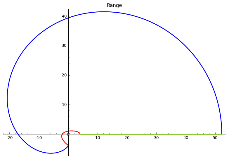
A graphic depiction of the convergence problems we run into when trying to evaluate the sum over the $c_n$. For the elliptic curve $E: y^2 + y = x^3 - 79*x + 342$ the above plot shows the cumulative sum $\sum_{n<T} c_n n^{-1/4}$ for $T$ up to 100000; this corresponds to $\Delta=4$. Note that even when we include this many terms in the sum, its value still varies considerably. It's unlikely the final computed value is correct to a single decimal digit yet.

A BETTER APPROACH (THE ONE IMPLEMENTED IN MY CODE)


We can get around this impasse by evaluating a modified sum over the zeros, one which requires us to only ever need to compute finitely many of the $c_n$. Here's how we do it. Start with the sum $\sum_{\gamma} \frac{s}{s^2+\gamma^2}$, and divide by $s^2$ to get $\frac{1}{s(s^2+\gamma^2)}$. Now hearken back to your college sophomore math classes and take the inverse Laplace transform of this sum. We get
$$ \mathcal{L}^{-1} \left[\sum_{\gamma} \frac{1}{s(s^2+\gamma^2)}\right](t) = \sum_{\gamma} \mathcal{L}^{-1} \left[\frac{1}{s(s^2+\gamma^2)}\right](t) = \frac{t^2}{2} \sum_{\gamma} \left(\frac{\sin(\frac{t}{2}\gamma)}{\frac{t}{2}\gamma}\right)^2 $$
Letting $\Delta = \frac{t}{2\pi}$ we get the sum
$$ \mathcal{L}^{-1} \left[\sum_{\gamma} \frac{s}{s^2+\gamma^2}\right](\Delta) = 2\pi^2\Delta^2 \sum_{\gamma} \text{sinc}^2(\Delta\gamma), $$
where $\text{sinc}(x) = \frac{\sin(\pi x)}{\pi x}$, and $\text{sinc}(0) = 1$.

Note that as before, $\text{sinc}^2(\Delta\gamma)$ exaluates to 1 for the central zeros, and is small but positive for all nonzero $\gamma$ when $\Delta$ is large. So again, this sum will give an upper bound on the analytic rank of $E$, and that this bound converges to the true analytic rank as $\Delta \to \infty$.

If we do the same - divide by $s^2$ and take inverse Laplace transforms - to the quantities on the right, we get the following:

  • $\mathcal{L}^{-1} \left[\frac{C_0}{s^2} \right] = 2\pi\Delta C_0;$
  • $ \mathcal{L}^{-1} \left[\sum_{k=1}^{\infty} \frac{1}{sk(k+s)}\right] = \sum_{k=1}^{\infty} \frac{1}{k^2}\left(1-e^{-2\pi\Delta k}\right);$
  • $\mathcal{L}^{-1} \left[ \sum_{n=1}^{\infty} c_n \frac{n^{-s}}{s^2} \right] = \sum_{\log n<2\pi\Delta} c_n\cdot(2\pi\Delta - \log n). $
Note that the last sum is finite: for any given value of $\Delta$, we only need to compute the $c_n$ for $n$ up to $e^{2\pi\Delta}$. This is the great advantage here: we can compute the sum exactly without introducing any truncation error. The other two quantities are also readly computable to any precision.

Combining the above values and dividing by $2\pi^2\Delta^2$, we arrive at the rank bounding formula which is implemented in my GSoC code, hideous as it is:
\begin{align*}
r < \sum_{\gamma} \text{sinc}^2(\Delta\gamma) =  \frac{1}{\pi\Delta} &\left[ C_0 + \frac{1}{2\pi\Delta}\sum_{k=1}^{\infty} \frac{1}{k^2}\left(1-e^{-2\pi\Delta k}\right) \right. \\
&\left. + \sum_{n<e^{2\pi\Delta}} c_n\left(1 - \frac{\log n}{2\pi\Delta}\right) \right] \end{align*}
Of course, the number of terms needed on the right hand side is still exponential in $\Delta$, so this limits the tightness of the sum we can compute on the left hand side. In practice a personal computer can compute the sum with $\Delta=2$ in a few seconds, and a more powerful cluster can handle $\Delta=3$ in a similar time. Beyond Delta values of about 4, however, the number of $c_n$ is just too great to make the sum effectively computable.

THE DENSITY OF ZEROS ON THE CRITICAL LINE


Explicit formula-type sums can also be used to answer questions about the distribution of zeros of $L_E$ along the critical line. Let $T$ be a positive real number, and $M_E(T)$ be the counting function that gives the number of zeros in the critical strip with imaginary part at most $T$ in magnitude. By convention, when $T$ coincides with a zero of $L_E$, then we count that zero with weight. In other words, we can write
$$ M_E(T) = \sum_{|\gamma|<T} 1 + \sum_{|\gamma|=T} 1/2.$$
There is a more mathematically elegant way to write this sum. Let $\theta(x)$ be the Heaviside function on $x$ given by
$$ \theta(x) = \begin{cases} 0, & x<0 \\
\frac{1}{2}, & x=0 \\
1, & x>0. \end{cases}$$
Then we have that
$$M_E(T) = \sum_{\gamma} \theta(T^2-\gamma^2). $$
We have written $M_E(T)$ as a sum over the zeros of $L_E$, so we expect that it comprises the left-hand-side of some explicit formula-type sum. This is indeed this the case. Using Fourier transforms we can show that
$$M_E(T) = \frac{2}{\pi}\left[C_0 T + \sum_{k=1}^{\infty} \left(\frac{T}{k} - \arctan \frac{T}{k}\right) + \sum_{n=1}^{\infty} \frac{c_n}{\log n}\cdot \sin(T\log n) \right] $$

With this formula in hand we can start asking questions on how the zeros of $L_E$ are distributed. For example, how does average zero density on the critical line scale as a function of $T$, the imaginary part of the area in the critical strip we're considering? How does zero density scale with the curve's conductor $N$?

If one assumes the Generalized Riemann Hypothesis, we can show that $\sum_{n=1}^{\infty} \frac{c_n}{\log n}\cdot \sin(T\log n) = O(\log T)$. Moreover, this sum is in a sense equidistributed about zero, so we expect its contribution for a sufficiently large randomly chosen value of $T$ to be zero. The other two quantities are more straightforward. The $C_0 T$ term is clearly linear in $T$. Going back to the definition of $C_0$, we see that $C_0 T = \frac{1}{2}T\log N + $constant$\cdot T$. Finally, we can show that the sum over $k$ equals $T\log T + O(\log T)$. Combining this gives us the estimate
$$ M_E(T) = \frac{1}{\pi} T (\log N + 2\log T+a) + O(\log T) $$
for some explicitly computable constant $a$ independent of $E$, $N$ or $T$ . That is, the number of zeros with imaginary part at most $T$ in magnitude is "very close" to $\frac{1}{\pi}T(\log N + 2\log T)$. Another way to put it is than the number of zeros in the interval $[T,T+1]$ is about $\frac{1}{2}\log N + \log T$.

The value of $M_E(T)$ for $T$ up to 30, for the elliptic curve $E: y^2 + y = x^3 - x$. The black line is just the 'smooth part' of $M_E(T)$, given by $\frac{2}{\pi}\left(C_0 T + \sum_{k=1}^{\infty} \left(\frac{T}{k} - \arctan \frac{T}{k}\right)\right)$. This gives us the 'expected number of zeros up to $T$', before we know any data about $E$ other than its conductor. The blue line is what we get when we add in $\sum_{n=1}^{\infty} \frac{c_n}{\log n}\cdot \sin(T\log n)$, which tells us the exact locations of the zeros: they will be found at the places where the blue curve jumps by 2.

Note that the sum over $n$ converges *very* slowly. To produce the above plot, I included terms up to $n=1 000 000$, and there is still considerable rounding visible in the blue curve. If I could some how evaluate the $c_n$ sum in all its infinite glory, then resulting plot would be perfectly sharp, comprised of flat lines that jump vertically by 2 at the loci of the zeros.


These are two of the uses of explicit formula-type sums in the context of elliptic curve $L$-functions. If you want to read more about them, feel free to pick up my PhD thesis - when it eventually gets published!

Vince Knight: Pointing at a blog post about Sage and a treasure hunt

$
0
0
It looks like I might be moving... I've been playing with jekyll + github and really love the workflow so it looks like I might be moving this blog over there.

It's not official yet as I still need to think about a couple of things but in the meantime here's a post I just wrote over there about how the team I was in used Sage in a mathematical treasure hunt: http://goo.gl/iLgGnL
Viewing all 414 articles
Browse latest View live