Well, Mid-Terms have just finished(I passed!), and I’ve been neglecting this blog so here are some updates. The app is now in beta! More info can be found at the sage-devel post here Most of the work done is internal, but there are a few external fixes and enhancements as well. Agendas for the next […]
↧
Nikhil Peter: GSoC – Post Mid-Term Update
↧
Simon Spicer: The Birch and Swinnerton-Dyer Conjecture and computing analytic rank
Let $E$ be an elliptic curve with $L$-function $L_E(s)$. Recall that Google Summer of Code project is to implement in Sage a method that allows us to compute $\sum_{\gamma} f(\Delta \gamma)$, where $\gamma$ ranges over the imaginary parts of the nontrivial zeros of $L_E$, $\Delta$ is a given positive parameter, and $f(x)$ is a specified symmetric continuous integrable function that is 1 at the origin. The value of this sum then bounds the analytic rank of $E$ - the number of zeros at the central point - from above, since we are summing $1$ with multipliticy $r_{an}$ in the sum, along with some other nonzero positive terms (that are hopefully small). See this post for more info on the method.
One immediate glaring issue here is that zeros that are close to the critical point will contribute values that are close to 1 in the sum, so the curve will then appear to have larger analytic rank than it actually does. An obvious question, then, is to ask: how close can the noncentral zeros get to the central point? Is there some way to show that they cannot be too close? If so, then we could figure out just how large of a $\Delta$ we would need to use in order to get a rank bound that is actually tight.
 |
| The rank zero curve $y^2 = x^3 - x^3 - 7460362000712 x - 7842981500851012704$ has an extremely low-lying zero at $\gamma = 0.0256$ (and thus another one at $-0.0256$; as a result the zero sum looks like it's converging towards a value of 2 instead of the actual analytic rank of zero. In order to actually get a sum value out that's less than one we would have to use a $\Delta$ value of about 20; this is far beyond what's feasible due to the exponential dependence of the zero sum method on $\Delta$. |
The good news is that there is hope in this regard; the nature of low-lying zeros for elliptic curve $L$-functions is actually the topic of my PhD dissertation (which I'm still working on, so I can't provide a link thereto just yet!). In order to understand how close the lowest zero can get to the central point we will need to talk a bit about the BSD Conjecture.
The Birch and Swinnerton-Dyer Conjecture is one of the two Clay Math Millenium Problems related to $L$-functions. The conjecture is comprised of two parts; the first part I mentioned briefly in this previous post. However, we can use the second part to gain insight into how good our zero sum based estimate for analytic rank will be.
Even though I've stated the first part of the BSD Conjecture before, for completeness I'll reproduce the full conjecture here. Let $E$ be an elliptic curve defined over the rational numbers, e.g. a curve represented by the equation $y^2 = x^3 + Ax + B$ for some integers $A$ and $B$ such that $4A^3+27B^2 \ne 0$. Let $E(\mathbb{Q})$ be the group of rational points on the elliptic curve, and let $r_{al}$ be the algebraic rank of $E(\mathbb{Q})$. Let $L_E(s)$ be the $L$-function attached to $E$, and let $L_E(1+s) = s^{r_{an}}\left[a_0 + a_1 s + \ldots\right]$ be the Taylor expansion of $L_E(s)$ about $s=1$ such that the leading coefficient $a_0$ is nonzero; $r_{an}$ is called the analytic rank of $E$ (see here for more details on all of the above objects). The first part of the BSD conjecture asserts that $r_{al}=r_{an}$; that is, the order of vanishing of the $L$-function about the central point is exactly equal to the number of free generators in the group of rational points on $E$.
The second part of the conjecture asserts that we actually know the exact value of that leading coefficient $a_0$ in terms of other invariants of $E$. Specifically:
$$ a_0 = \frac{\Omega_E\cdot\text{Reg}_E\cdot\prod_p c_p\cdot\#\text{Ш}(E/\mathbb{Q})}{(\#E_{\text{Tor}}(\mathbb{Q}))^2}. $$
Fear not if you have no idea what any of these quantities are. They are all things that we know how to compute - or at least estimate in size. I provide below brief descriptions of each of these quantities; however, feel free to skip this part. It suffices to know that we have a formula for computing the exact value of that leading coefficient $a_0$.
- $\#E_{\text{Tor}}(\mathbb{Q})$ is the number of rational torsion points on $E$. Remember that the solutions $(x,y)$ to the elliptic curve equation $y^2 = x^3 + Ax+B$, where $x$ and $y$ are both rational numbers, form a group. Recall also that that the group of rational points $E(\mathbb{Q})$ may be finite or infinite, depending on whether the group has algebraic rank zero, or greater than zero. However, it turns out that there are only ever finitely many torsion points - those which can be added to themselves some finite number of times to get the group identity element. These points of finite order form a subgroup, denoted $E_{\text{Tor}}(\mathbb{Q})$, and the quantity in question is just the size of this finite group (squared in the formula). In fact, it's been proven that the size of $E_{\text{Tor}}(\mathbb{Q})$ is at most 16.
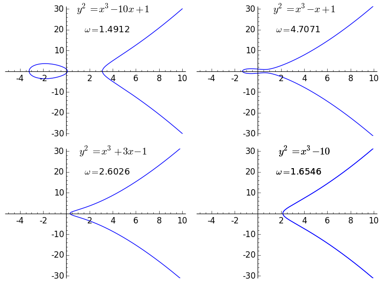
- $\Omega_E$ is the real period of $E$. This is perhaps a bit more tricky to define, but it essentially is a number that measures the size of the set of real points of $E$. If you plot the graph of the equation representing $E: y^2 = x^3 + Ax + B$ on the cartesian plane, you get something that looks like one of the following:
![]()
The plots of the real solutions to four elliptic curves, and their associated real periods.
There is a way to assign an intrinsic "size" to these graphs, which we denote the real period $\Omega_E$. The technical definition is that $\Omega_E$ is equal to the integral of the absolute value of the differential $\omega = \frac{dx}{2y}$ along the part of the real graph of $E$ that is connected to infinity (that or twice that depending on whether the cubic equation $x^3 + Ax + B$ has one or three real roots respectively). - $\text{Reg}_E$ is the regulator of $E$. This is a number that measures the "density" of rational points on $E$. Recall that $E(\mathbb{Q}) \approx T \times \mathbb{Z}^{r_{an}}$, i.e there free part of $E(\mathbb{Q})$ is isomorphic to $r_{an}$ copies of the integers. There is a canonical way to embed the free part of $E(\mathbb{Q})$ in $\mathbb{R}^{r_{an}}$ as a lattice; the regulator $\text{Reg}_E$ is the volume of the fundamental domain of this lattice. The thing to take away here is that elliptic curves with small regulators have lots of rational points whose coefficients have small numerators and denominators, while curves with large regulators have few such points.
- $\prod_p c_p$ is the Tamagawa product for $E$. For each prime $p$, one can consider the points on $E$ over the $p$-adic numbers $\mathbb{Q}_p$. The Tamagawa number $c_p$ is the ratio of the size of the full group of $p$-adic points on $E$ to the subgroup of $p$-adic points that are connected to the identity. This is always a positive integer, and crucially, in all but a finite number of cases the ratio is 1. Thus we can consider the product of the $c_p$ as we range over all prime numbers, and this is precisely the definition of the Tamagawa product.
- $\#\text{Ш}(E/\mathbb{Q})$ is the order of the Tate-Shafarevich group of $E$ over the rational numbers. The Tate-Shafarevich group of $E$ is probably the most mysterious part of the BSD formula; it is defined as the subgroup of the Weil–Châtelet group $H^1(G_{\mathbb{Q}},E)$ that becomes trivial when passing to any completion of $\mathbb{Q}$. If you're like me then this definition will be completely opaque; however, we can think of $\text{Ш}(E/\mathbb{Q})$ as measuring how much $E$ violates the local-global principle: that one should be able to find rational solutions to an algebraic equation by finding solutions modulo a prime number $p$ for each $p$, and then piecing this information together with the Chinese Remainder Theorem to get a rational solution. Curves with nontrivial $\text{Ш}$ have homogeneous spaces that have solutions modulo $p$ for all $p$, but no rational points. The main thing here is that $\text{Ш}$ is conjectured to be finite, in which case $\#\text{Ш}(E/\mathbb{Q})$ is just a positive integer (in fact, it can be shown for elliptic curves that if $\text{Ш}$ is indeed finite, then its size is a perfect square).
Why is the BSD Conjecture relevant to rank estimation? Because it helps us overcome the crucial obstacle to computing analytic rank exactly: without extra knowledge, it's impossible to decide using numerical techniques whether the $n$th derivative of the $L$-function at the central point is exactly zero, or just so small that it looks like it is zero to the precision that we're using. If we can use the BSD formula to show a priori that $a_0$ must be at least $M_E$ in magnitude, where $M_E$ is some number that depends only on some easily computable data attached to the elliptic curve $E$, then all we need to do is evaluate successive derivatives of $L_E$ at the central point to enough precision to decide if that derivative is less than $M_E$ or not; this is readily doable on a finite precision machine. Keep going until we hit a derivative which is then definitely greater than $M_E$ in magnitude, at which we can halt and declare that the analytic rank is precisely the order of that derivative.
In the context of the explicit formula-based zero sum rank estimation method implemented in our GSoC project, the size of the leading coefficient also controls how far close the lowest noncentral zero can be from the central point. Specifically, we have the folling result: Let $\gamma_0$ be the lowest-lying noncentral zero for $L_E$ (i.e. the zero closest to the central point that is not actually at the central point); let $\Lambda_E(s) = N^{s/2}(2\pi)^s\Gamma(s)L_E(s)$ is the completed $L$-function for $E$, and let $\Lambda_E(1+s) = s^{r_{an}}\left[b_0 + b_1 s + b_2 s^2 \ldots\right]$ be the Taylor expansion of $\Lambda_E$ about the central point. Then:
$$ \gamma_0 > \sqrt{\frac{b_0}{b_2}}. $$
Thankfully, $b_0$ is easily relatable back to the constant $a_0$, and we have known computable upper bounds on the magnitude of $b_2$, so knowing how small $a_0$ is tells us how close the lowest zero can be to the central point. Thus bounding $a_0$ from below in terms of some function of $E$ tells us how large of a $\Delta$ value we need to use in our zero sum, and thus how long the computation will take as a function of $E$.
If this perhaps sounds a bit handwavy at this point it's because this is all still a work in progress, to be published as part of my dissertation. Nevertheless, the bottom line is that bounding the leading $L$-series coefficient from below gives us a way to directly analyze the computational complexity of analytic rank methods.
I hope to go into more detail in a future post about what we can do to bound from below the leading coefficient of $L_E$ at the central point, and why this is a far from straightforward endeavour.
↧
↧
Nikhil Peter: Sage Android – UI Update
It’s been a busy week so far in the land of UI improvements. Disclaimer: I’m pretty bad at UI, so any and all suggestions are welcome. Firstly, last week’s problems have been resolved viz. Everything is saved nicely on orientation change, including the interacts, which required quite a bit of effort. In short, it involved […]
↧
Liang Ze: The Group Ring and the Regular Representation
In the previous post, we saw how to decompose a given group representation into irreducibles. But we still don’t know much about the irreducible representations of a (finite) group. What do they look like? How many are there? Infinitely many?
In this post, we’ll construct the group ring of a group. Treating this as a vector space, we get the regular representation, which turns out to contain all the irreducible representations of $G$!
The group ring $FG$
Given a (finite) group $G$ and a field $F$, we can treat each element of $G$ as a basis element of a vector space over $F$. The resulting vector space generated by $g \in G$ is
Let’s do this is Sage with the group $G = D_4$ and the field $F = \mathbb{Q}$:
(The Sage cells in this post are linked, so things may not work if you don’t execute them in order.)
We can view $v \in FG$ as vector in $F^n$, where $n$ is the size of $G$ :
Here, we’re treating each $g \in G$ as a basis element of $FG$
Vectors in $FG$ are added component-wise:
Multiplication as a linear transformation
In fact $FG$ is also a ring (called the group ring), because we can multiply vectors using the multiplication rule of the group $G$:
That wasn’t very illuminating. However, treating multiplication by $v \in FG$ as a function
one can check that each $T_v$ is a linear transformation! We can thus represent $T_v$ as a matrix whose columns are $T_v(g), g \in G$:
The regular representation
We’re especially interested in $T_g, g \in G$. These are invertible, with inverse $T_{g^{-1}}$, and their matrices are all permutation matrices, because multiplying by $g \in G$ simply permutes elements of $G$:
Define a function $\rho_{FG}$ which assigns to each $g\in G$ the corresponding $T_g$:
Then $(FG,\rho_{FG})$ is the regular representation of $G$ over $F$.
The regular representation of any non-trivial group is not irreducible. In fact, it is a direct sum of all the irreducible representations of $G$! What’s more, if $(V,\rho)$ is an irreducible representation of $G$ and $\dim V = k$, then $V$ occurs $k$ times in the direct-sum decomposition of $FG$!
Let’s apply the decomposition algorithm in the previous post to $(FG,\rho_{FG})$ (this might take a while to run):
So the regular representation of $D_4$ decomposes into four (distinct) $1$-dim representations and two (isomorphic) $2$-dim ones.
Building character
We’ve spent a lot of time working directly with representations of a group. While more concrete, the actual matrix representations themselves tend to be a little clumsy, especially when the groups in question get large.
In the next few posts, I’ll switch gears to character theory, which is a simpler but more powerful way of working with group representations.
↧
Vince Knight: This class teaches me to not trust my classmates: An iterated prisoners dilemma in class
On Monday, in class we played an iterated prisoner’s dilemma tournament. I have done this many times (both in outreach events with Paul Harper and in this class). This is always a lot of fun but none more so than last year when Paul’s son Thomas joined us. You can read about that one here.
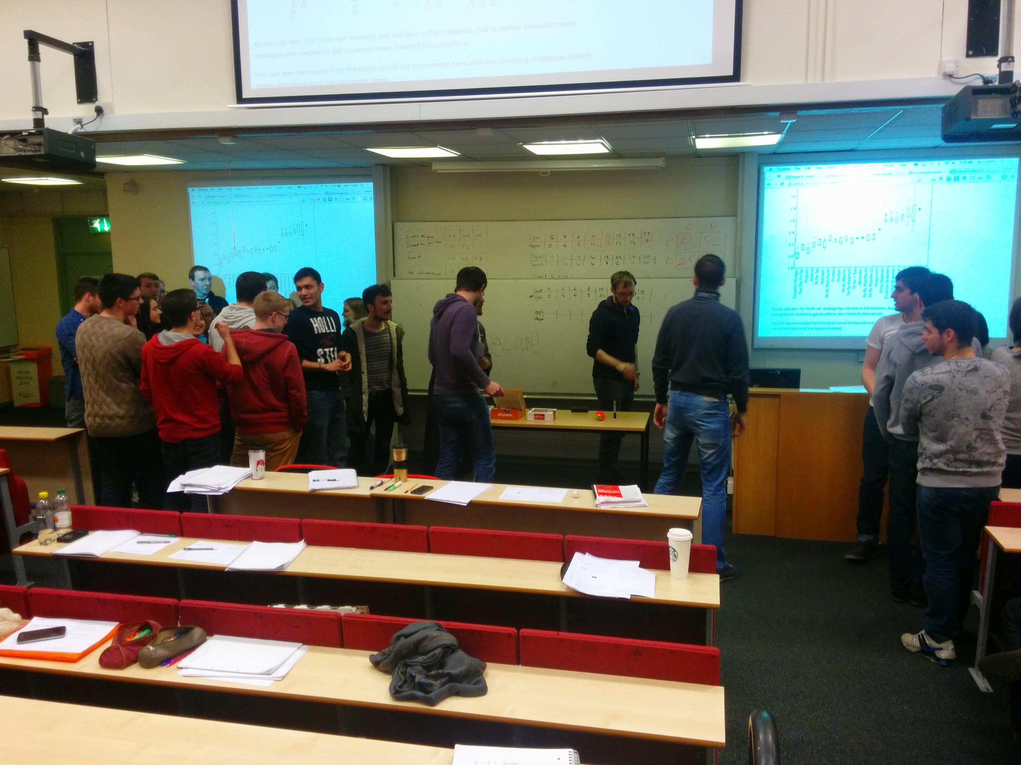
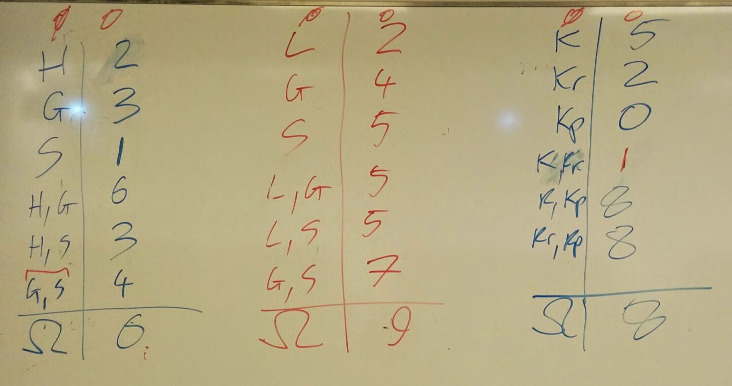
The format of the game is as close to that of Axelrod’s original tournament as I think it can be. I split the class in to 4 teams and we create a round robin where each team plays every other team at 8 consecutive rounds of the prisoner’s dilemma:
The utilities represent ‘years in prison’ and over the 3 matches that each team will play (against every other team) the goal is to reduce the total amount of time spent in prison.
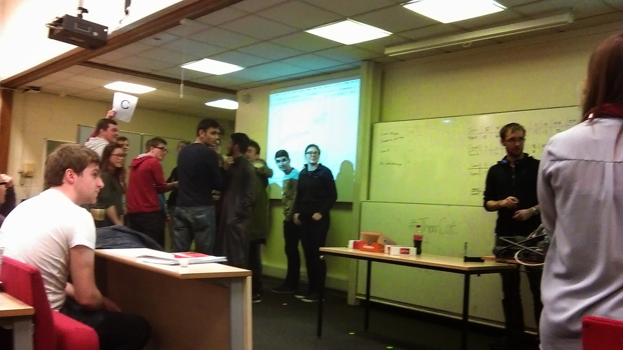
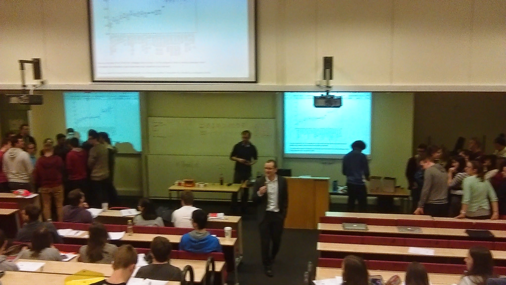
Here are some photos from the game:
Here are the scores:
We see that ‘We will take the gun’ acquired the least total score and so they won the collection of cookies etc…
(The names followed a promise from me to let the team with the coolest name have a nerf gun… Can’t say this had the wanted effect…)
At one point during the tournament, one team actually almost declared a strategy which was cool:
We will cooperate until you defect at which point we will reevaluate
This was pretty cool as I hadn’t discussed at all what a strategy means in a repeated game (ie I had not discussed the fact that a strategy in a repeated game takes count of both play histories).
Here are all the actual duels:
You’ll also notice at the end that a coalition formed and one team agreed to defect so that they could share the prize. This happens about 50% of the time when we play this game but I never cease to be amused by it. Hopefully everyone found this fun and perhaps some even already agree with a bit of feedback I received on this course last year:
‘This class teaches me to not trust my classmates’
One of the other really cool things that happened after this class was H asking for a hand to submit a strategy to my Axelrod repository. She built a strategy called ‘Once Bitten’ that performs pretty well! You can see it here (click on ‘Blame’ and you can see the code that she wrote).
(Big thanks to Jason for keeping track of the scores and to Geraint for helping and grabbing some nice pictures)
↧
↧
Sébastien Labbé: Arnoux-Rauzy-Poincaré sequences
In a recent article with Valérie Berthé [BL15], we provided a multidimensional continued fraction algorithm called Arnoux-Rauzy-Poincaré (ARP) to construct, given any vector \(v\in\mathbb{R}_+^3\), an infinite word \(w\in\{1,2,3\}^\mathbb{N}\) over a three-letter alphabet such that the frequencies of letters in \(w\) exists and are equal to \(v\) and such that the number of factors (i.e. finite block of consecutive letters) of length \(n\) appearing in \(w\) is linear and less than \(\frac{5}{2}n+1\). We also conjecture that for almost all \(v\) the contructed word describes a discrete path in the positive octant staying at a bounded distance from the euclidean line of direction \(v\).
In Sage, you can construct this word using the next version of my package slabbe-0.2 (not released yet, email me to press me to finish it). The one with frequencies of letters proportionnal to \((1, e, \pi)\) is:
sage: from slabbe.mcf import algo
sage: D = algo.arp.substitutions()
sage: it = algo.arp.coding_iterator((1,e,pi))
sage: w = words.s_adic(it, repeat(1), D)
word: 1232323123233231232332312323123232312323...
The factor complexity is close to 2n+1 and the balance is often less or equal to three:
sage: w[:10000].number_of_factors(100)
202
sage: w[:100000].number_of_factors(1000)
2002
sage: w[:1000].balance()
3
sage: w[:2000].balance()
3
Note that bounded distance from the euclidean line almost surely was proven in [DHS2013] for Brun algorithm, another MCF algorithm.
Other approaches: Standard model and billiard sequences
Other approaches have been proposed to construct such discrete lines.
One of them is the standard model of Eric Andres [A03]. It is also equivalent to billiard sequences in the cube. It is well known that the factor complexity of billiard sequences is quadratic \(p(n)=n^2+n+1\) [AMST94]. Experimentally, we can verify this. We first create a billiard word of some given direction:
sage: from slabbe import BilliardCube
sage: v = vector(RR, (1, e, pi))
sage: b = BilliardCube(v)
sage: b
Cubic billiard of direction (1.00000000000000, 2.71828182845905, 3.14159265358979)
sage: w = b.to_word()
sage: w
word: 3231232323123233213232321323231233232132...
We create some prefixes of \(w\) that we represent internally as char*. The creation is slow because the implementation of billiard words in my optional package is in Python and is not that efficient:
sage: p3 = Word(w[:10^3], alphabet=[1,2,3], datatype='char')
sage: p4 = Word(w[:10^4], alphabet=[1,2,3], datatype='char') # takes 3s
sage: p5 = Word(w[:10^5], alphabet=[1,2,3], datatype='char') # takes 32s
sage: p6 = Word(w[:10^6], alphabet=[1,2,3], datatype='char') # takes 5min 20s
We see below that exactly \(n^2+n+1\) factors of length \(n<20\) appears in the prefix of length 1000000 of \(w\):
sage: A = ['n'] + range(30)
sage: c3 = ['p_(w[:10^3])(n)'] + map(p3.number_of_factors, range(30))
sage: c4 = ['p_(w[:10^4])(n)'] + map(p4.number_of_factors, range(30))
sage: c5 = ['p_(w[:10^5])(n)'] + map(p5.number_of_factors, range(30)) # takes 4s
sage: c6 = ['p_(w[:10^6])(n)'] + map(p6.number_of_factors, range(30)) # takes 49s
sage: ref = ['n^2+n+1'] + [n^2+n+1 for n in range(30)]
sage: T = table(columns=[A,c3,c4,c5,c6,ref])
sage: T
  n    p_(w[:10^3])(n)   p_(w[:10^4])(n)   p_(w[:10^5])(n)   p_(w[:10^6])(n)   n^2+n+1
+----+-----------------+-----------------+-----------------+-----------------+---------+
  0    1                 1                 1                 1                 1
  1    3                 3                 3                 3                 3
  2    7                 7                 7                 7                 7
  3    13                13                13                13                13
  4    21                21                21                21                21
  5    31                31                31                31                31
  6    43                43                43                43                43
  7    52                55                56                57                57
  8    63                69                71                73                73
  9    74                85                88                91                91
  10   87                103               107               111               111
  11   100               123               128               133               133
  12   115               145               151               157               157
  13   130               169               176               183               183
  14   144               195               203               211               211
  15   160               223               232               241               241
  16   176               253               263               273               273
  17   192               285               296               307               307
  18   208               319               331               343               343
  19   224               355               368               381               381
  20   239               392               407               421               421
  21   254               430               448               463               463
  22   268               470               491               507               507
  23   282               510               536               553               553
  24   296               552               583               601               601
  25   310               596               632               651               651
  26   324               642               683               703               703
  27   335               687               734               757               757
  28   345               734               787               813               813
  29   355               783               842               871               871
Billiard sequences generate paths that are at a bounded distance from an euclidean line. This is equivalent to say that the balance is finite. The balance is defined as the supremum value of difference of the number of apparition of a letter in two factors of the same length. For billiard sequences, the balance is 2:
sage: p3.balance()
2
sage: p4.balance() # takes 2min 37s
2
Other approaches: Melançon and Reutenauer
Melançon and Reutenauer [MR13] also suggested a method that generalizes Christoffel words in higher dimension. The construction is based on the application of two substitutions generalizing the construction of sturmian sequences. Below we compute the factor complexity and the balance of some of their words over a three-letter alphabet.
On a three-letter alphabet, the two morphisms are:
sage: L = WordMorphism('1->1,2->13,3->2')
sage: R = WordMorphism('1->13,2->2,3->3')
sage: L
WordMorphism: 1->1, 2->13, 3->2
sage: R
WordMorphism: 1->13, 2->2, 3->3
Example 1: periodic case \(LRLRLRLRLR\dots\). In this example, the factor complexity seems to be around \(p(n)=2.76n\) and the balance is at least 28:
sage: from itertools import repeat, cycle
sage: W = words.s_adic(cycle((L,R)),repeat('1'))
sage: W
word: 1213122121313121312212212131221213131213...
sage: map(W[:10000].number_of_factors, [10,20,40,80])
[27, 54, 110, 221]
sage: [27/10., 54/20., 110/40., 221/80.]
[2.70000000000000, 2.70000000000000, 2.75000000000000, 2.76250000000000]
sage: W[:1000].balance()  # takes 1.6s
21
sage: W[:2000].balance()  # takes 6.4s
28
Example 2: \(RLR^2LR^4LR^8LR^{16}LR^{32}LR^{64}LR^{128}\dots\) taken from the conclusion of their article. In this example, the factor complexity seems to be \(p(n)=3n\) and balance at least as high (=bad) as \(122\):
sage: W = words.s_adic([R,L,R,R,L,R,R,R,R,L]+[R]*8+[L]+[R]*16+[L]+[R]*32+[L]+[R]*64+[L]+[R]*128,'1')
sage: W.length()
330312
sage: map(W.number_of_factors, [10, 20, 100, 200, 300, 1000])
[29, 57, 295, 595, 895, 2981]
sage: [29/10., 57/20., 295/100., 595/200., 895/300., 2981/1000.]
[2.90000000000000,
 2.85000000000000,
 2.95000000000000,
 2.97500000000000,
 2.98333333333333,
 2.98100000000000]
sage: W[:1000].balance()  # takes 1.6s
122
sage: W[:2000].balance()  # takes 6s
122
Example 3: some random ones. The complexity \(p(n)/n\) occillates between 2 and 3 for factors of length \(n=1000\) in prefixes of length 100000:
sage: for _ in range(10):
....:     W = words.s_adic([choice((L,R)) for _ in range(50)],'1')
....:     print W[:100000].number_of_factors(1000)/1000.
2.02700000000000
2.23600000000000
2.74000000000000
2.21500000000000
2.78700000000000
2.52700000000000
2.85700000000000
2.33300000000000
2.65500000000000
2.51800000000000
For ten randomly generated words, the balance goes from 6 to 27 which is much more than what is obtained for billiard words or by our approach:
sage: for _ in range(10):
....:     W = words.s_adic([choice((L,R)) for _ in range(50)],'1')
....:     print W[:1000].balance(), W[:2000].balance()
12 15
8 24
14 14
5 11
17 17
14 14
6 6
19 27
9 16
12 12
References
| [BL15] | V. Berthé, S. Labbé, Factor Complexity of S-adic words generated by the Arnoux-Rauzy-Poincaré Algorithm, Advances in Applied Mathematics 63 (2015) 90-130. http://dx.doi.org/10.1016/j.aam.2014.11.001 |
| [DHS2013] | Delecroix, Vincent, Tomás Hejda, and Wolfgang Steiner. “Balancedness of Arnoux-Rauzy and Brun Words.” In Combinatorics on Words, 119–31. Springer, 2013. http://link.springer.com/chapter/10.1007/978-3-642-40579-2_14. |
| [A03] | E. Andres, Discrete linear objects in dimension n: the standard model, Graphical Models 65 (2003) 92-111. |
| [AMST94] | P. Arnoux, C. Mauduit, I. Shiokawa, J. I. Tamura, Complexity of sequences defined by billiards in the cube, Bull. Soc. Math. France 122 (1994) 1-12. |
| [MR13] | G. Melançon, C. Reutenauer, On a class of Lyndon words extending Christoffel words and related to a multidimensional continued fraction algorithm. J. Integer Seq. 16, No. 9, Article 13.9.7, 30 p., electronic only (2013). https://cs.uwaterloo.ca/journals/JIS/VOL16/Reutenauer/reut3.html |
↧
Vince Knight: Playing an infinitely repeated game in class
Following the iterated Prisoner’s dilemma tournament my class I and I played last week we went on to play a version of the game where we repeated things infinitely many times. This post will briefly describe what we got up to.
As you can read in the post about this activity from last year, the way we play for an infinite amount of time (that would take a while) is to apply a discounting factor \(\delta\) to the payoffs and to interpret this factor as the probability with which the game continues.
Before I go any further (and put up pictures with the team names) I need to explain something (for the readers who are not my students).
For every class I teach I insist in spending a fair while going over a mid module feedback form that is used at Cardiff University (asking students to detail 3 things they like and don’t like about the class). One student wrote (what is probably my favourite piece of feedback ever):
“Vince is a dick… but in a good way.”
Anyway, I mentioned that to the class during my feedback-feedback session and that explains one of the team names (which I found pretty amusing):
- Orange
- Where’s the gun
- We don’t know
- Vince is a good dick
Once we had the team names set up (and I stopped trying to stop laughing) I wrote some quick Python code that we could run after each iteration:
importrandomcontinue_prob=.5ifrandom.random()<continue_prob:print'Game continues'else:print'Game Over'We started off by playing with (\delta=.5) and here are the results:
You can see the various duels here:
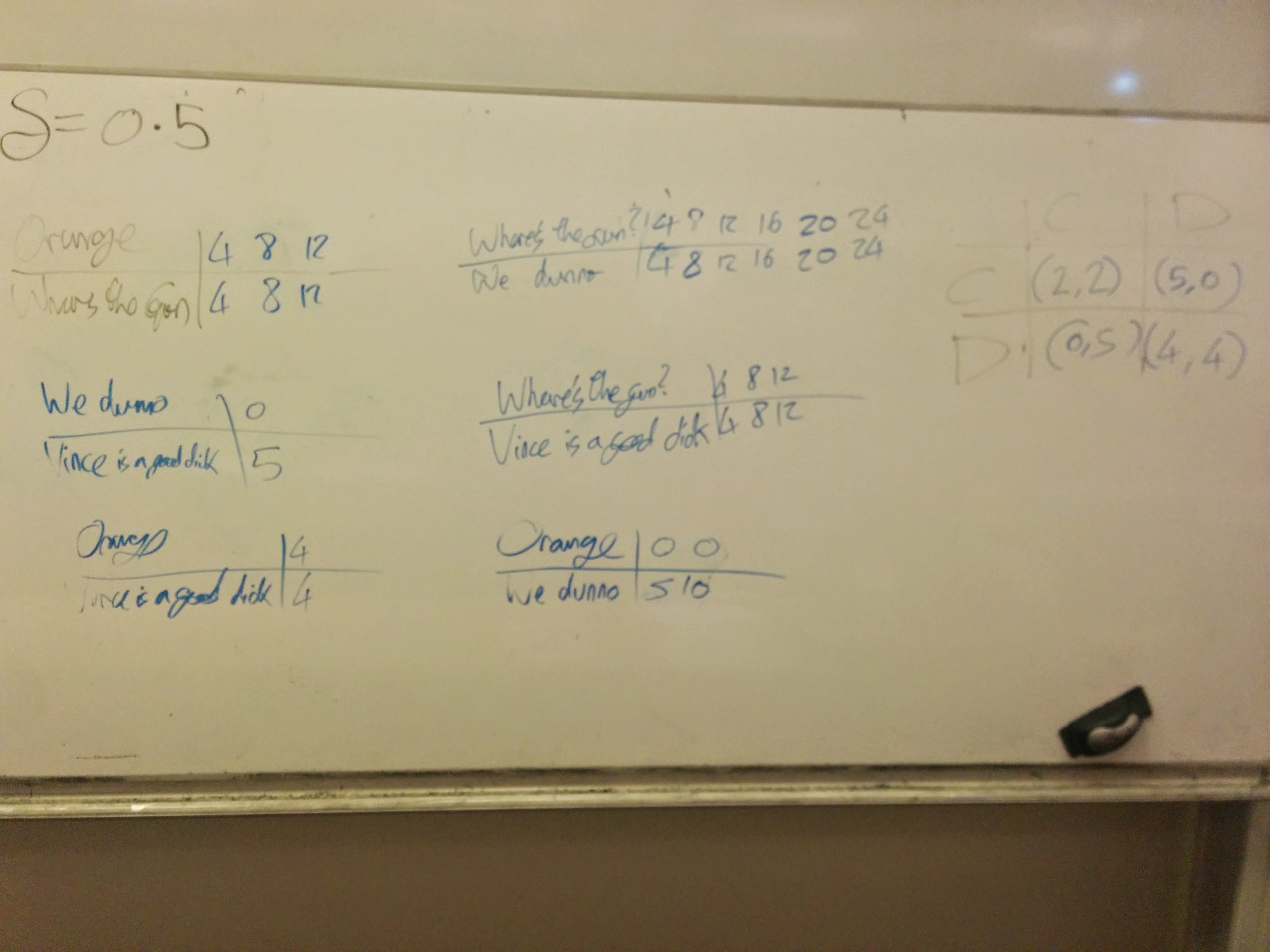
As you can see, very little cooperation happened this way and in fact because everyone could see what everyone else was doing Orange took advantage of the last round to create a coalition and win. We also see one particular duel that cost two teams very highly (because the ‘dice rolls’ did not really help).
After this I suggest to the class that we play again but that no one got to see what was happening to the other teams (this was actually suggested to me by students the year before). We went ahead with this and used \(delta=.25\): so the game had a less chance of carrying on.
You can see the result and duels here (this had to be squeezed on to a board that could be hidden):
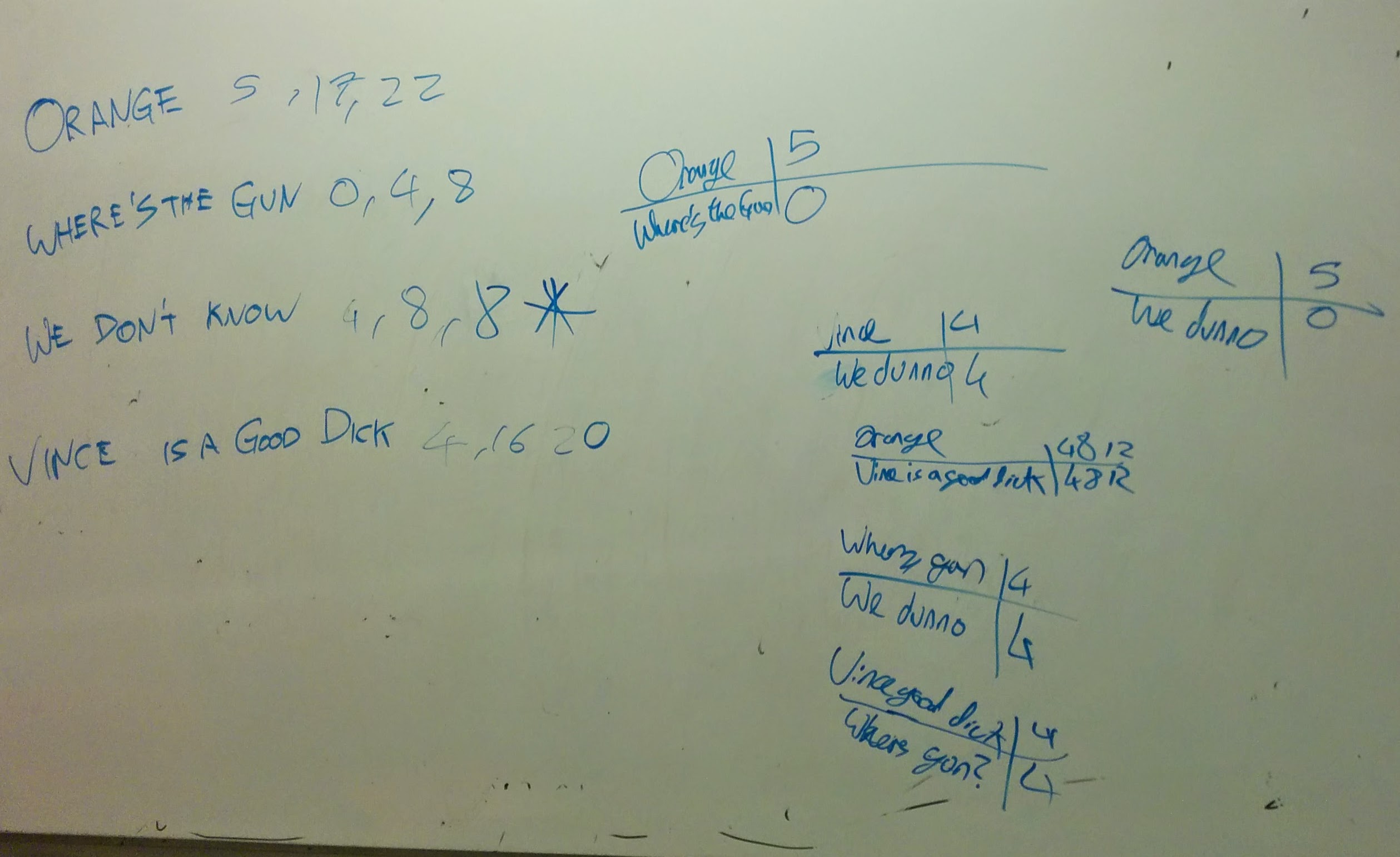
Based on the theory we would expect more cooperation to be likely but as you can see this did not happen.
The tie at the end was settled with a game of Rock Paper Scissors Lizard Spock which actually gave place to a rematch of the Rock Paper Scissors Lizard Spock tournament we played earlier. Except this time Laura, lost her crown :)
↧
Liang Ze: Animated GIFs
I really should be posting about character theory, but I got distracted making some aesthetic changes to this blog (new icon and favicon!) and creating animations like this:
I’m not putting this in a SageCell because this could take quite a while, especially if you increase the number of frames (by changing the parameters in srange), but feel free to try it out on your own copy of Sage. It saves an animated GIF that loops forever (iterations = 0) at the location specified by savefile.
For more information, checkout the Sage reference for animated plots.
↧
Vince Knight: Discussing the game theory of walking/driving in class
Last week, in game theory class we looked at pairwise contest games. To introduce this we began by looking at the particular game that one could use to model the situation of two individuals walking or driving towards each other:
The above models people walking/driving towards each other and choosing a side of the road. If they choose the same side they will not walk/drive in to each other.
I got a coupe of volunteers to simulate this and ‘walk’ towards each other having picked a side. We very quickly arrived at one of the stage Nash equilibria: both players choosing left and/or choosing right.
I wrote a blog post about this a while ago when the BBC wrote an article about social convention. You can read that here.
We went on to compute the evolutionary stability of 3 potential stable equilibria:
- Everyone driving on the left;
- Everyone driving on the right;
- Everyone randomly picking a side each time.
Note that the above corresponds to the three Nash equilibria of the game itself. You can see this using some Sage code immediately (here is a video I just put together showing how one can use Sage to obtain Nash equilibria) - just click on ‘Evaluate’:
We did this calculations in two ways:
- From first principles using the definitions of evolutionary stability (this took a while). 2 Using a clever theoretic result that in effect does the analysis for us once and for all.
Both gave us the same result: driving on a given side of the road is evolutionarily stable whereas everyone randomly picking a side is not (a nudge in any given direction would ensure people picked a side).
This kind of corresponds to the two (poorly drawn) pictures below:

To further demonstrate the instability of the ‘choose a random side’ situation here is a plot of the actual evolutionary process (here is a video that shows what is happening):
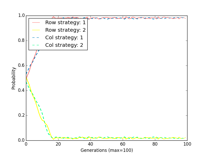
We see that if we start by walking randomly the tiniest of mutation send everyone to picking a side.
↧
↧
Vince Knight: Incomplete information games in class
Last week my class and I looked at the basics of games with incomplete information. The main idea is that players do not necessarily know where there are in an extensive form game. We repeated a game I played last year that you can read about here.
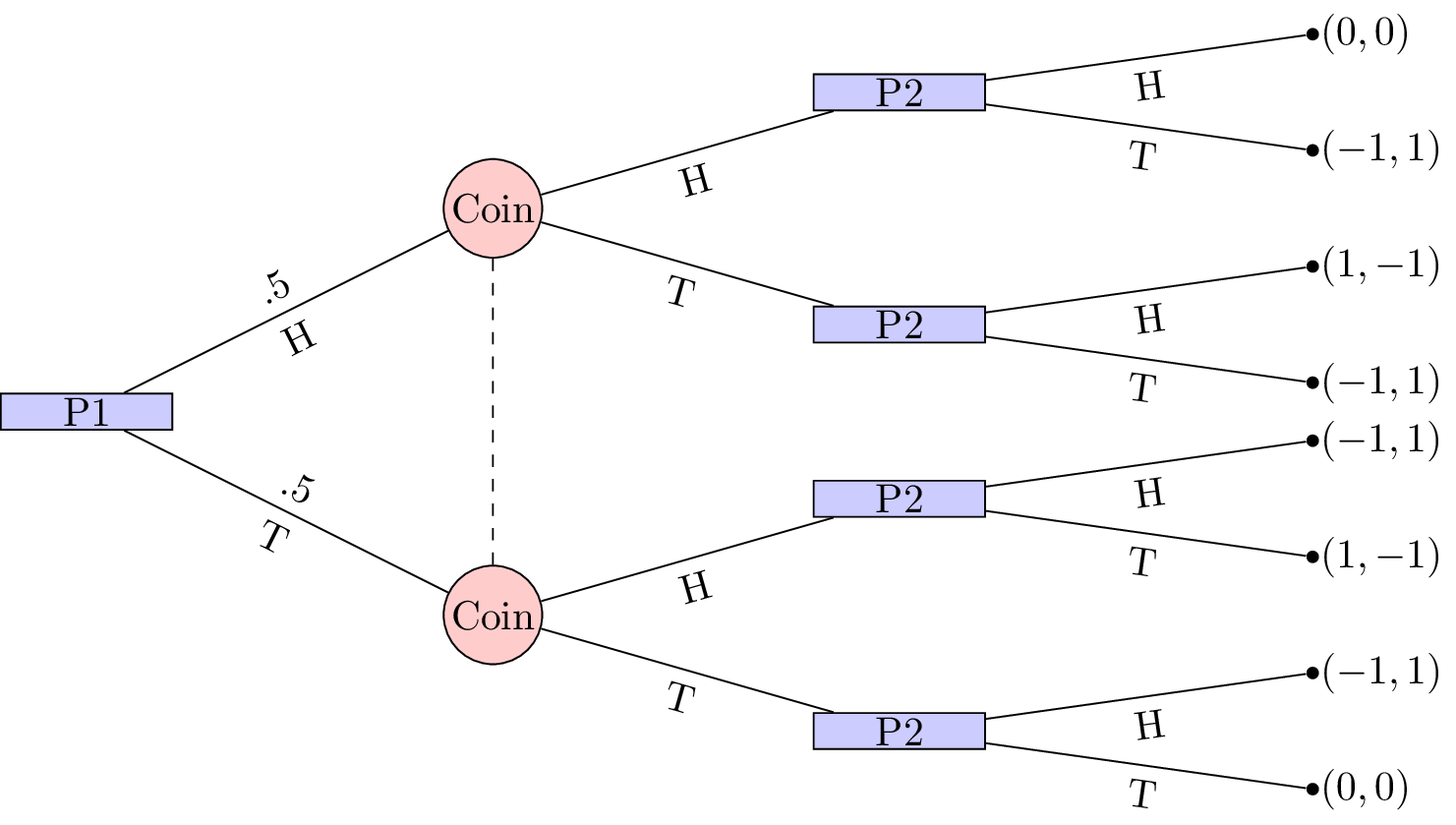
Here is a picture of the game we played (for details take a look at the post from last year):
We played a round robing where everyone played against everyone else and you can see the results in these two notebook pages that Jason kept track off:
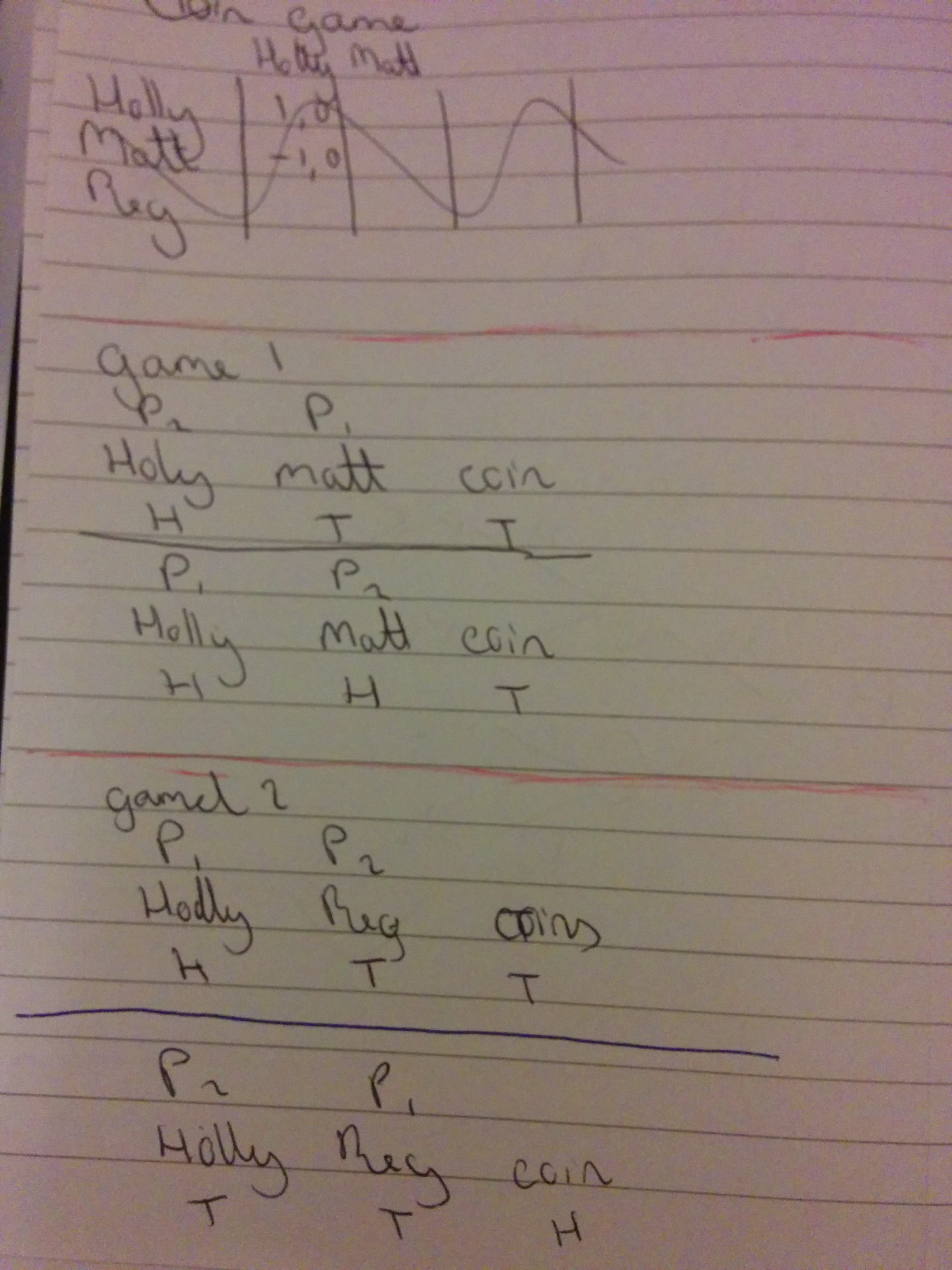
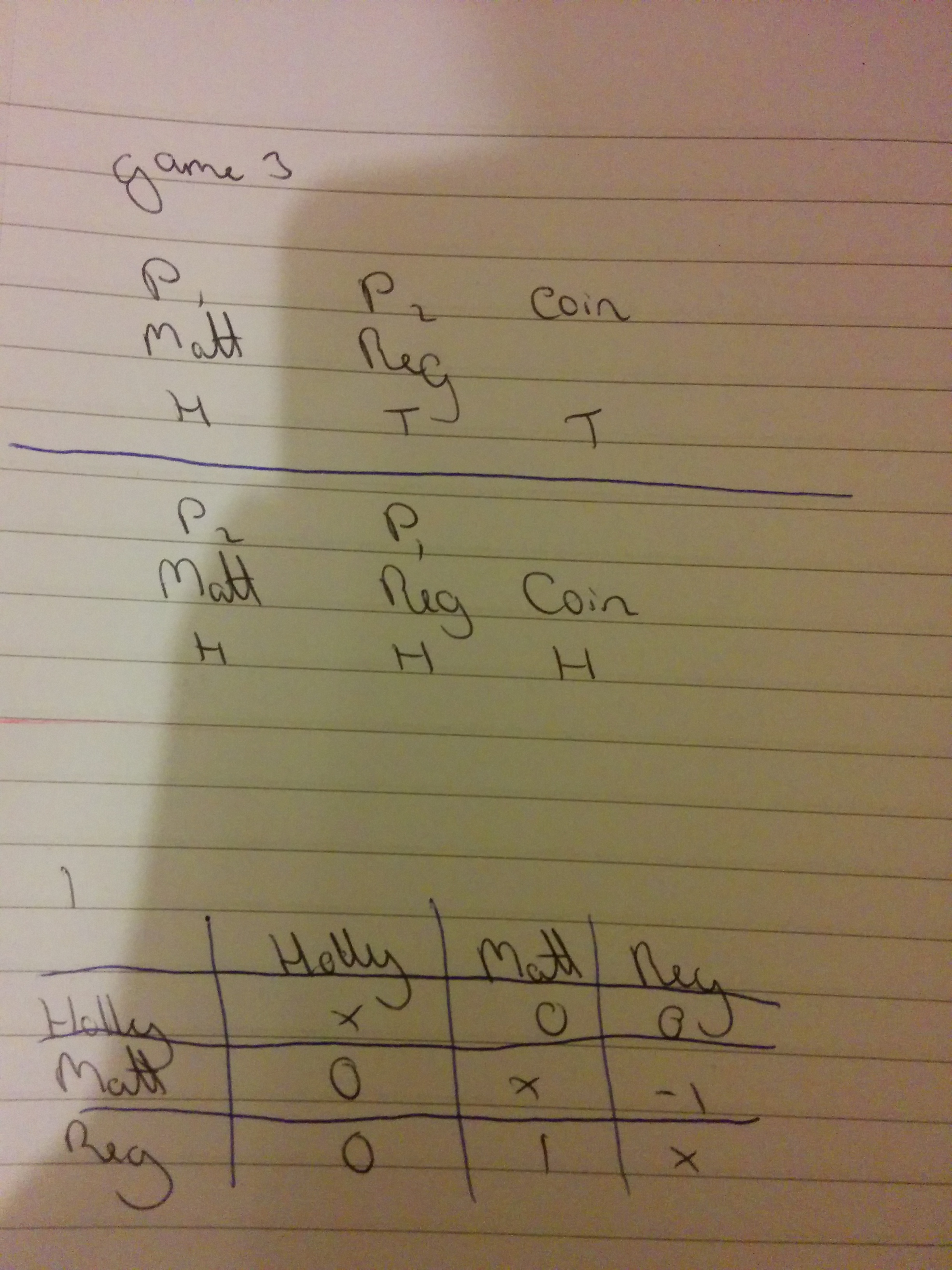
We see that the winner was Reg, who on both occasions of being the second player: went with the coin.
To find the Nash equilibria for this game we can translate it in to normal form game by doing the following two things:
- Identify the strategy sets for the players
- Averaging of the outcome probabilities
This gives the following strategies:
and
The strategies for the second player correspond to a 2-vector indexed by the information sets of the second player. In other words the first letter says what to do if the coin comes up as heads and the second letter says what to do if the coin comes up as tails:
- \(HH\): No matter what: play heads;
- \(HT\): If the coin comes up as heads: play heads. If the coin comes up as tails: play tails.
- \(TH\): If the coin comes up as heads: play tails. If the coin comes up as tails: play heads.
- \(TT\): No matter what: play tails;
Once we have done that and using the above ordering we can obtain the normal form game representation:
In class we obtained the Nash equilibria for this game by realising that the third column strategy (\(TH\): always disagree with the coin) was dominated and then carrying out some indifference analysis.
Here let us just throw it at Sage (here is a video showing and explaining some of the code):
The equilibria returned confirms what we did in class: the first player can more or less randomly (with bounds on the distribution) pick heads or tails but the second player should always agree with the coin.
↧
Vince Knight: Playing stochastic games in class
The final blog post I am late in writing is about the Stochastic game we played in class last week. The particular type of game I am referring to is also called a Markov game where players play a series of Normal Form games, with the next game being picked from a random distribution the nature of which depends on the strategy profiles. In other words the choice of the players does not only impact on the utility gained by the players but also on the probability of what the net game will be… I blogged about this last year so feel free to read about some of the details there.
The main idea is that one stage game corresponds to this normal form game (a prisoner’s dilemma):
at the other we play:
The probability distributions, of the form \((x,1-x)\) where \(x\) is the probability with which we play the first game again are given by:
and the probability distribution for the second game was \((0,1)\). In essence the second game was an absorption game and so players would try and avoid it.
To deal with the potential for the game to last for ever we played this with a discounting factor \(\delta=1/2\). Whilst that discounting factor will be interpreted as such in theory, for the purposes of playing the game in class we used that as a probability at which the game continues.
You can see a photo of this all represented on the board:

We played this as a team game and you can see the results here:

As opposed to last year no actual duel lasted more than one round: I had a coded dice to sample at each step. The first random roll of the dice was to see if the game continued based on the \(\delta\) property (this in effect ‘deals with infinity’). The second random sample was to find out which game we payed next and if we ever went to the absorption games things finished there.
The winner was team B who in fact defected after the initial cooperation in the first game (perhaps that was enough to convince other teams they would be cooperative).
After playing this, we calculated (using some basic algebra examining each potential pure equilibria) the Nash equilibria for this game and found that there were two pure equilibria: both players Cooperating and both players defecting.
↧
Liang Ze: Character Theory Basics
This post illustrates some of SageMath’s character theory functionality, as well as some basic results about characters of finite groups.
Basic Definitions and Properties
Given a representation $(V,\rho)$ of a group $G$, its character is a map $ \chi: G \to \mathbb{C}$ that returns the trace of the matrices given by $\rho$:
A character $\chi$ is irreducible if the corresponding $(V,\rho)$ is irreducible.
Despite the simplicity of the definition, the (irreducible) characters of a group contain a surprising amount of information about the group. Some big theorems in group theory depend heavily on character theory.
Let’s calculate the character of the permutation representation of $D_4$. For each $g \in G$, we’ll display the pairs:
(The Sage cells in this post are linked, so things may not work if you don’t execute them in order.)
Many of the following properties of characters can be deduced from properties of the trace:
- The dimension of a character is the dimension of $V$ in $(V,\rho)$. Since $\rho(\text{Id})$ is always the identity matrix, the dimension of $\chi$ is $\chi(\text{Id})$.
- Because the trace is invariant under similarity transformations, $\chi(hgh^{-1}) = \chi(g)$ for all $g,h \in G$. So characters are constant on conjugacy classes, and are thus class functions.
- Let $\chi_V$ denote the character of $(V,\rho)$. Recalling the definitions of direct sums and tensor products, we see that
The Character Table
Let’s ignore the representation $\rho$ for now, and just look at the character $\chi$:
This is succinct, but we can make it even shorter. From point 2 above, $\chi$ is constant on conjugacy classes of $G$, so we don’t lose any information by just looking at the values of $\chi$ on each conjugacy class:
Even shorter, let’s just display the values of $\chi$:
This single row of numbers represents the character of one representation of $G$. If we knew all the irreducible representations of $G$ and their corresponding characters, we could form a table with one row for each character. This is called the character table of $G$.
Remember how we had to define our representations by hand, one by one? We don’t have to do that for characters, because SageMath has the character tables of small groups built-in:
This just goes to show how important the character of a group is. We can also access individual characters as a functions. Let’s say we want the last one:
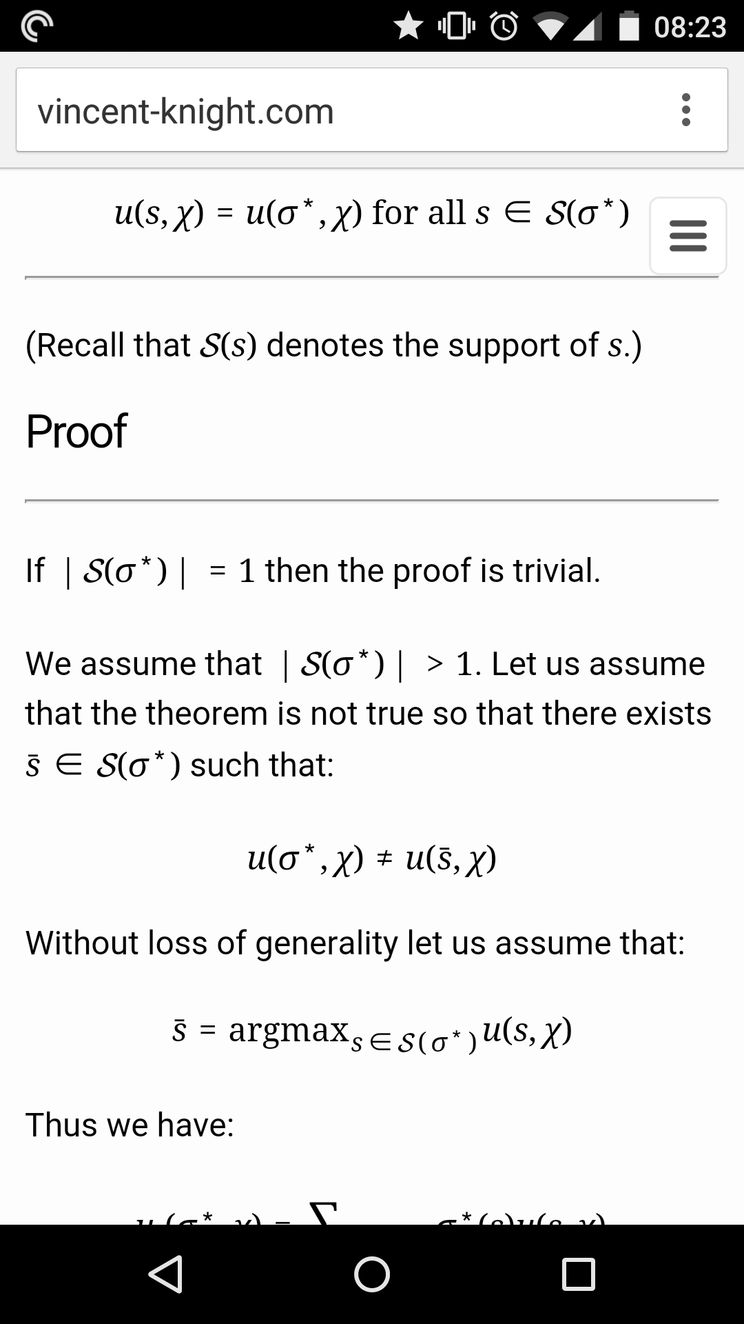
Notice that the character we were playing with, $[4,2,0,0,0]$, is not in the table. This is because its representation $\rho$ is not irreducible. At the end of the post on decomposing representations, we saw that $\rho$ splits into two $1$-dimensional irreducible representations and one $2$-dimensional one. It’s not hard to see that the character of $\rho$ is the sum of rows 1,4 and 5 in our character table:
Just as we could decompose every representation of $G$ into a sum of irreducible representations, we can express any character as a sum of irreducible characters.
The next post discusses how to do this easily, by making use of the Schur orthogonality relations. These are really cool relations among the rows and columns of the character table. Apart from decomposing representations into irreducibles, we’ll also be able to prove that the character table is always square!
↧
Vince Knight: Cooperative basketball in class
Today in class we repeated the game we played last year. 3 teams of 3 students took part this year and here is a photo of the aftermath:
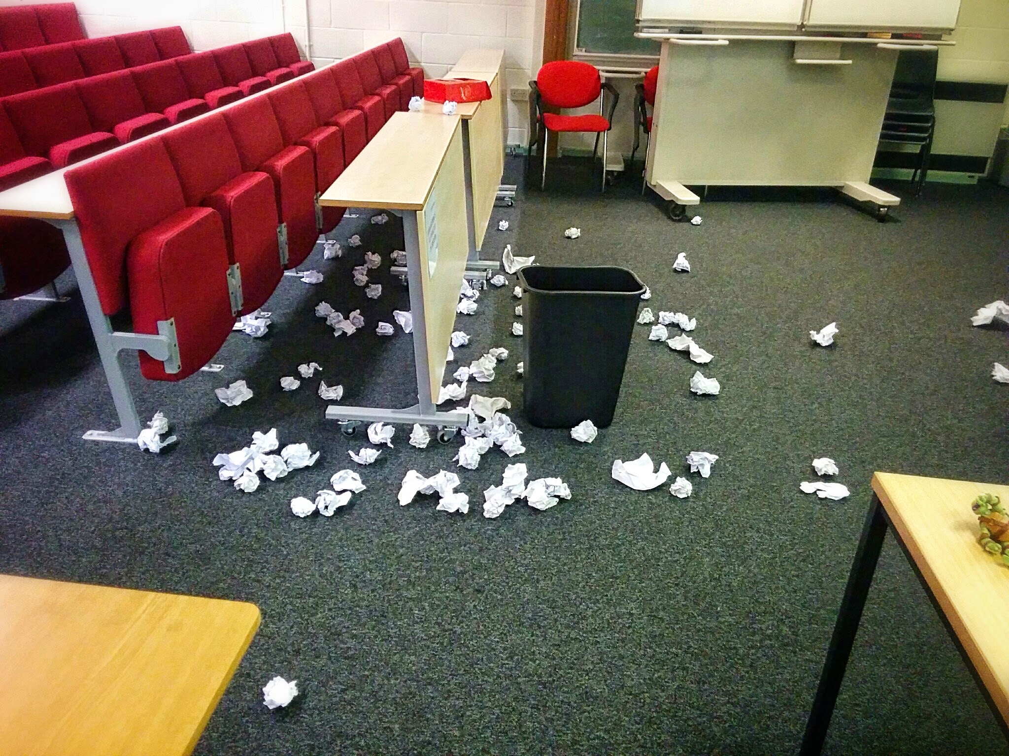
As a class we watched the three teams attempt to free-throw as many crumpled up pieces of paper in to the bin as possible.
Based on the total number we then tried to come up with how many each subset/coalition of players would have gotten in. So for example, 2 out of 3 of the teams had one student crumple paper while the other 2 took shots. So whilst that individual did not get any in, they contributed an important part to the team effort.
Here are the characteristic functions that show what each team did:
Here is some Sage code that gives the Shapley value for each game (take a look at my class notes or at last years post to see how to calculate this):
Let us define the first game:
If you click Evaluate above you see that the Shapley value is given by:
(This one we calculated in class)
By changing the numbers above we get the following for the other two games.
Game 2:
Game 3:
This was a bit of fun and most importantly from a class point of view gave us some nice numbers to work from and calculate the Shapley value together.
If anyone would like to read about the Shapley value a bit more take a look at the Sage documentation which not only shows how to calculate it using Sage but also goes over some of the mathematics (including another formulation).
↧
↧
Vince Knight: Marrying toys and students
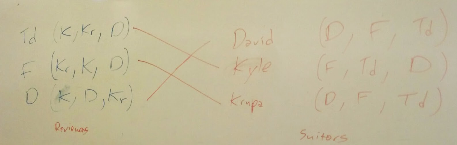
In class yesterday we took a look at matching games. These are sometimes referred to as stable marriage problems. To have some data for us to play with I asked for some volunteers to marry. Sadly I apparently am not allowed to ask students to rank each other in class and I also do not have the authority to marry. So, like last year I used some of my office toys and asked students to rank them.
I brought three toys to class:
- The best ninja turtle: Donatello
- A tech deck
- A foam football
I asked 3 students to come down and rank them and in turn I let the toys rank the students.
We discussed possible matchings with some great questions such as:
“Are we trying to make everyone as happy as possible?”
The answer to that is: no. We are simply trying to ensure that no one has an incentive to deviate from their current matching by breaking their match for someone they prefer and who also prefers them.
Here is the stable matching we found together:
Note that we can run the Gale-Shapley value using Sage:
The 3 students got to hold on to the toys for the hour and I was half expecting the football to be thrown around but sadly that did not happen. Perhaps next year.
↧
Vince Knight: A one week flipped learning environment to introduce Object Oriented Programming
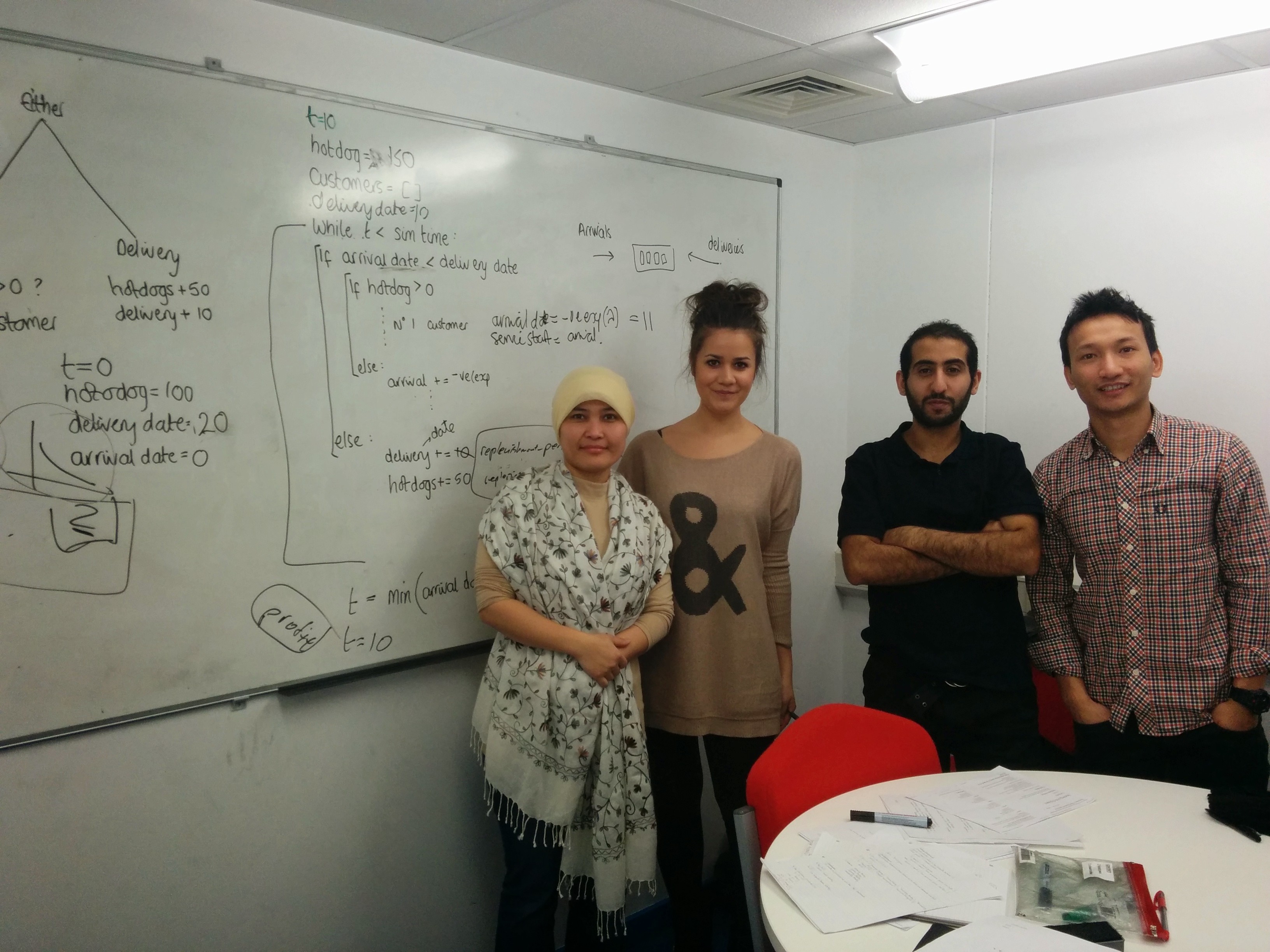
This post describes a teaching activity that is run for the Cardiff MSc. programmes. The activity is revolves around a two day hackathon that gets students to use Python and object oriented programming to solve a challenge. The activity is placed within a flipped learning environment and makes use of what I feel is a very nice form of assessment (we just get to know the students).
This year is the third installment of this exercise which came as a result of the MSc advisory board requesting that object oriented programming be introduced to our MSc.
Before describing the activity itself let me just put this simple diagram that describes the flipped learning environment here (if you would like more info about it be sure to talk to Robert Talbert who has always been very helpful to me):

Description of what happens
After 3 iterations and a number of discussions about the format with Paul Harper (the director of the MSc) I think the last iteration is pretty spot on and it goes something like this:
Monday: Transfer of content
We give a brief overview of Python (you can see the slides here) up until and including basic syntax for classes.
Tuesday + Wednesday: Nothing
Students can, if they want to, read up about Python, look through videos at the website and elsewhere, look through past challenges etc… This is in effect when the knowledge transfer happens
Thursday: Flying solo followed by feedback
Students are handed a challenge of some sort (you can see the past two here). Students work in groups of 4 at attempting to solve the problem. On this day, the two postgrads (Jason and Geraint) and myself observe the groups. When we are asked questions we in general ask questions back. This sometimes leads to a fair bit of frustration but is the difficult process that makes the rest of the process worthwhile.
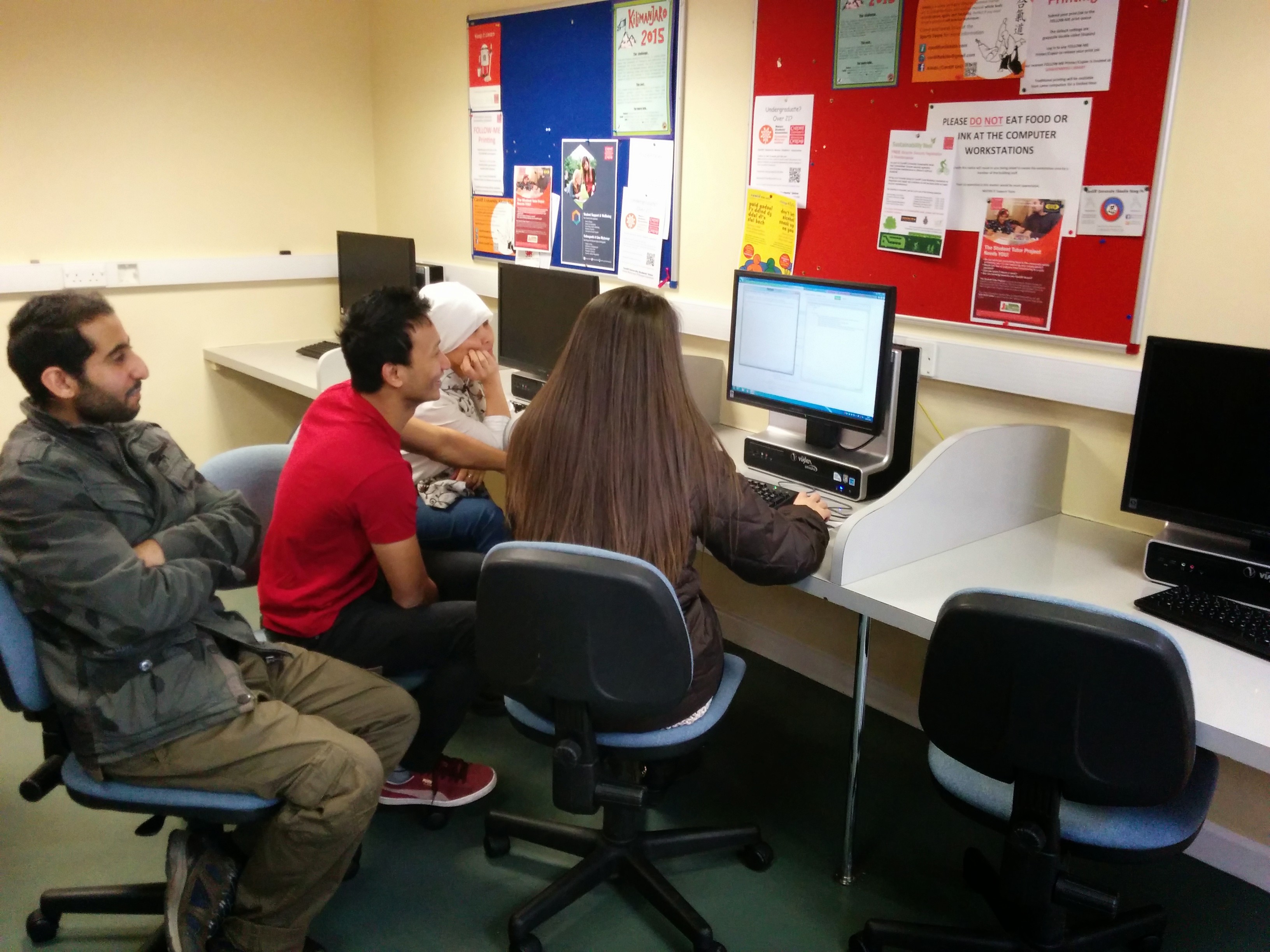
Here is a photo of some of the groups getting to work:
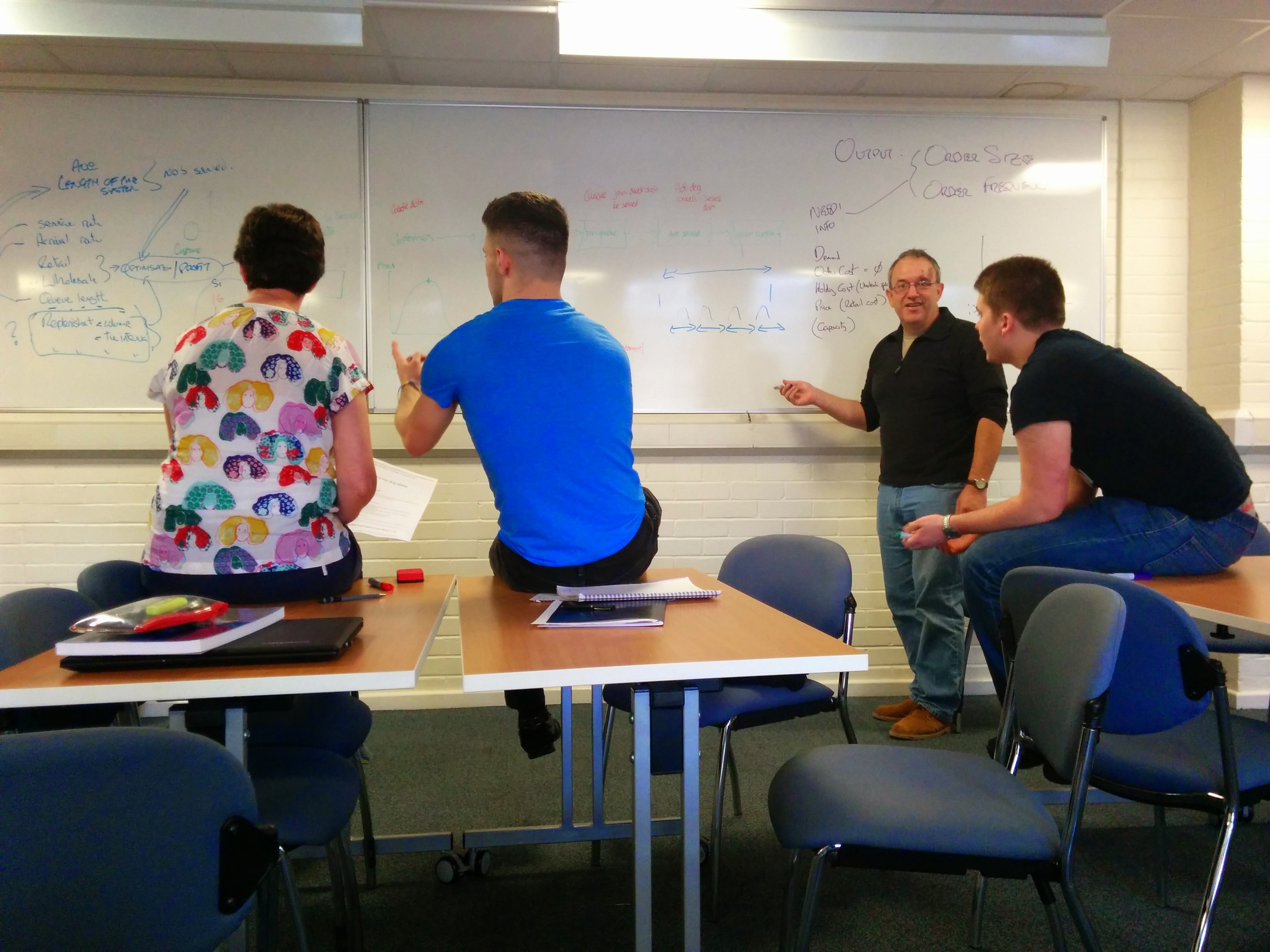
At the very end of the day (starting at 1600 for about 30 minutes with each group). During this feedback session go through the code written by each group in detail, highlighting things they are having difficulty with and agreeing on a course of action for the next day. This is the point at which the class ‘flips’ so to speak: transfer of content is done and difficulties are identified and conceptualised.
Here is a photo of Jason, Geraint and I at the end of a very long day after the feedback sessions:
The other point of this day is that we start our continuous assessment: taking notes and discussing how each group is doing:
- Where are they progress wise?
- What difficulties do we need to look out for?
- How are the groups approaching the problem and working together.
Here you can see a photo of Jason in front of the board that we fill up over the 2 days with notes and comments:

Friday: Sprint finish with more assistance
On the second/last day students are given slightly more assistance from Jason, Geraint and I but are still very much left to continue with their hard work. The main difference being that when students ask questions we sometimes answer them.
Here is one group who managed to crack something quite difficult on the second day:
The final part of this day is to round all the students together and announce the marks, which brings us nicely to the assessment part of this activity.
Assessment
I really enjoy assessing this activity. This is not something I say about assessment very often, but we are continuously assessing the students and are able to gain a true idea of how they do. The final piece of code is not what everything is marked on as it is in essence not terribly important.
Here is a photo of the team who did the best this year:
If I could sit with students over the 11 week period of the other courses I teach and get to know them and assess them that way, that is indeed how I would do it.
Summary
Here is a summary of how I feel this activity fits in the original diagram I had:

As you can see despite ‘being in contact’ with students for most of Thursday I would not consider this contact time in the usual sense as most of that contact is part of the assessment.
This is always a very fun (and exhausting) two days and I look forward to next year.
↧
Vince Knight: My 5 reasons why jekyll + github is a terrible teaching tool.
For the past year or so I have been using jekyll for all my courses. If you do not know, in a nutshell, jekyll is a ruby framework that lets you write templates for pages and build nice websites using static markdown files for your content. Here I will describe what I think of jekyll from a pedagogic point of view, in 5 main points.
1. Jekyll is terrible because the tutorial is too well written and easy to follow.
First of all, as an academic I enjoy when things are difficult to read and follow. The Jekyll tutorial can get you up and running with a jekyll site in less than 5 minutes. It is far too clear and easy to follow. This sort of clear and to the point explanation is very dangerous from a pedagogic point of view as students might stumble upon it and raise their expectations of the educational process they are going through.
In all seriousness, the tutorial is well written and clear, with a basic knowledge of the command line you can modify the base site and have a website deployed in less than 10 minutes.
2. Jekyll is terrible because it works too seamlessly with github.
First of all gh-pages takes care of the hosting. Not having to use a complicated server saves far too much time. As academics we have too much free time already, I do not like getting bored.
Github promotes the sharing and openness of code, resources and processes. Using a jekyll site in conjunction with github means that others can easily see and comment on all the materials as well as potentially improve them. This openness is dangerous as it ensures that courses are living and breathing things as opposed to a set of notes/problem sheets that sit safely in a drawer somewhere.
The fact that jekyll uses markdown is also a problem. On github anyone can easily read and send a pull request (which improves things) without really knowing markdown (let alone git). This is very terrible indeed, here for example is a pull request sent to me by a student. The student in question found a mistake in a question sheet and asked me about it, right there in the lab I just said ‘go ahead and fix it :)’ (and they did). Involving students in the process of fixing/improving their course materials has the potential for utter chaos. Furthermore normalising mistakes is another big problem: all students should be terrified of making a mistake and/or trying things.
Finally, having a personal site as a github project gives you a site at the following url:
username.github.io
By simply having a gh-pages branch for each class site, this will
automatically be served at:
username.github.io/class-site
This is far too sensible and flexible. Furthermore the promotion of decentralisation of content is dangerous. If one of my class sites breaks: none of my others will be affected!!! How can I expect any free time with such a robust system? This is dangerously efficient.
3. Jekyll is terrible because it is too flexible.
You can (if you want to) include:
A disqus.com board to a template for a page which means that students can easily comment and talk to you about materials. Furthermore you can also use this to add things to your materials in a discussion based way, for example I have been able to far too easily to add a picture of a whiteboard explaining something students have asked.
Mathjax. With some escaping this works out of the box. Being able to include nicely rendered mathematics misaligns students’ expectations as to what is on the web.
Sage cells can be easily popped in to worksheets allowing students to immediately use code to illustrate/explain a concept.
and various others: you can just include any html/javascript etc…
This promotion of interactive and modern resources by Jekyll is truly terrible as it gets students away from what teaching materials should really be about: dusty notes in the bottom of a drawer (worked fine for me).
The flexibility of Jekyll is also really terrible as it makes me forget the restrictions imposed on me by whatever VLE we are supposed to use. This is making me weak and soft, when someone takes the choice away from me and I am forced to use the VLE, I most probably won’t be ready.
(A jekyll + github setup also implis that a wiki immediately exists for a page and I am also experimenting with a gitter.im room for each class).
4. Jekyll is terrible because it gives a responsive site out of the box.
Students should consume their materials exactly when and how we want them to. The base jekyll site cames with a basic responsive framework, here is a photo of one of my class sheets (which also again shows the disgustingly beautifully rendered mathematics):
This responsive framework works right out of the box (you can also obviously use further frameworks if you want to, see my point about flexibility) from the tutorial and this encourages students to have access to the materials on whatever platform they want whenever they want. This cannot be a good thing.
5. Jekyll is terrible because it saves me too much time.
The main point that is truly worrying about jekyll is how much time it saves me. I have mentioned this before, as academics we need to constantly make sure we do not get bored. Jekyll does not help with this.
I can edit my files using whatever system I want (I can even do this on github directly if I wanted to), I push and the website is up to date.
In the past I would have a lot of time taken up by compiling a LaTeX document and uploading to our VLE. I would sit back and worry about being bored before realising (thankfully) that I had a typo and so needed to write, delete and upload again.
Furthermore, I can easily use the github issue tracker to keep on top of to do lists etc… (which I am actually beginning to do for more or less every aspect of my life). TAs can also easily fix/improve minor things without asking me to upload whatever it is they wrote.
Github + Jekyll works seamlessly and ensures that I have more time to respond to student queries and think. This time for reflection on teaching practice is dangerous: I might choose to do things differently than how they have been done for the past 100 years.
(In case my tone is unclear: I am such a huge jekyll fan and think it is a brilliant pedagogic tool. There might well be various other static site generators and other options so please do comment about them below :))
↧
Vince Knight: Code on cake, poker and a number theory classification web app
I have just finished writing feedback and obtaining marks for my first year students’ presentations. These presentations follow 11 weeks during which students formed companies and worked together to come up with a ‘product’ which had to involve mathematics and code (this semester comes just after 11 weeks of learning Python and Sage). In this post I’ll briefly describe some of the great things that the students came up with.
I must say that I was blown away by the standard this year. Last year the students did exceptionally well but this year the standard was even higher, I am so grateful for the effort put in by more or less everyone.
Some of the great projects included:
A website that used a fitted utility function (obtained from questioning family, friends, flatmates) to rank parking lots in terms of price and distance from a given venue (the website was written in Django and the function fitted using Sage).
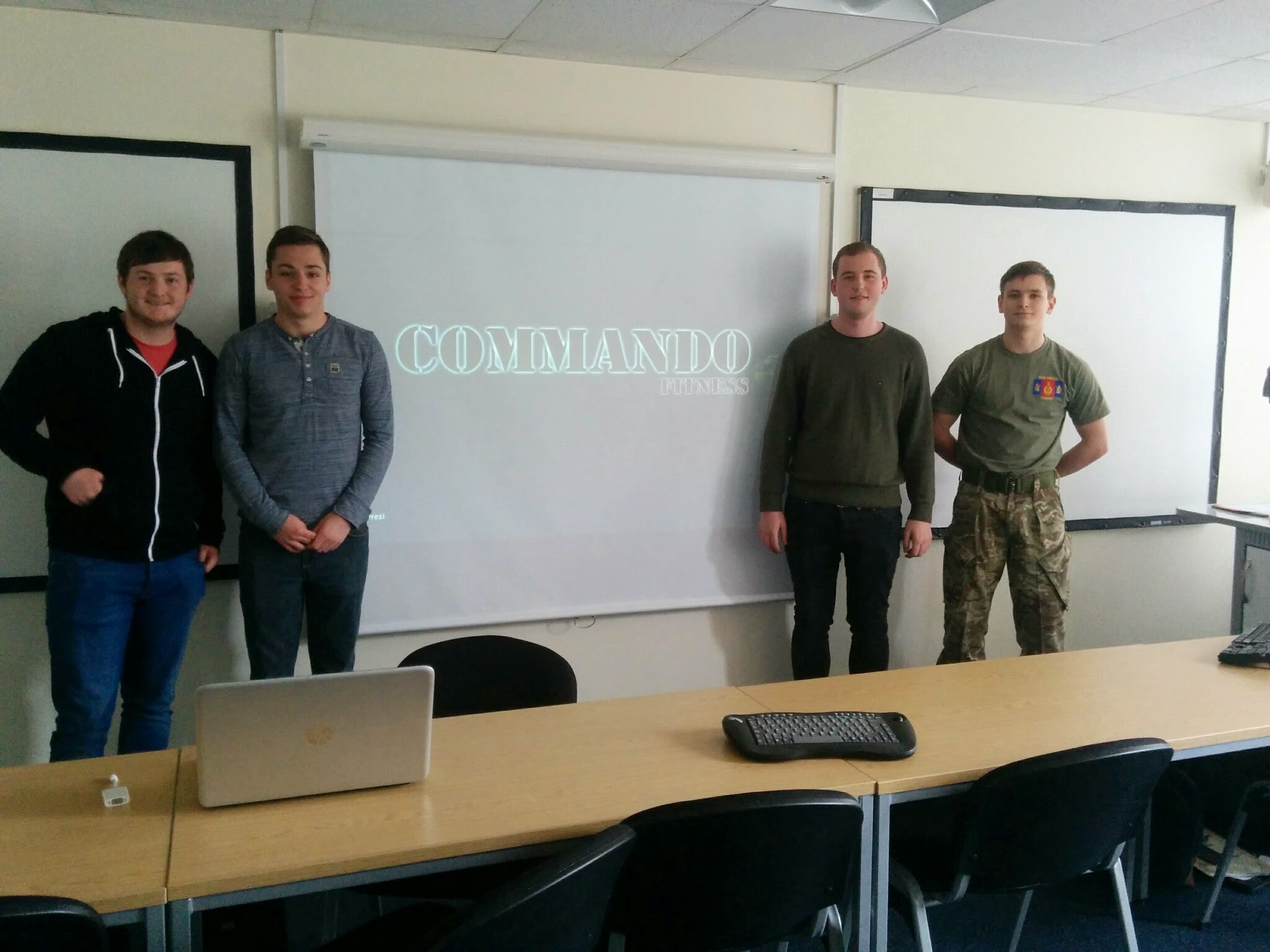
A commando training app, with an actual reservist marine who is a student of ours:
![]()
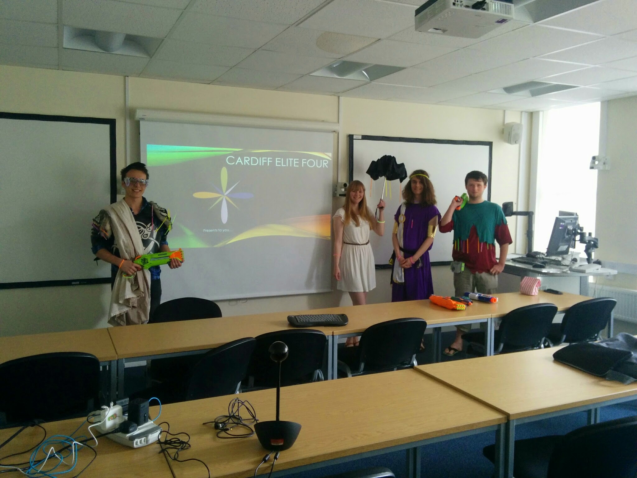
A story based game with an original storyline stemming from the zodiac. The presentation culminated in Geraint, Jason and I (who were the audience) retaliating to their Nerf gun attack with our (hidden under the desk) Nerf guns (we had a hunch that this group would ambush us…). The game mechanics itself was coded in pure Python and the UI was almost written in Django (that was the goal but they didn’t have the time to fully implement it).
![]()
A Django site that had a graphical timeline of mathematics (on click you had access to a quizz and info etc…). This was one I was particularly excited about as it’s a tool I would love to use.
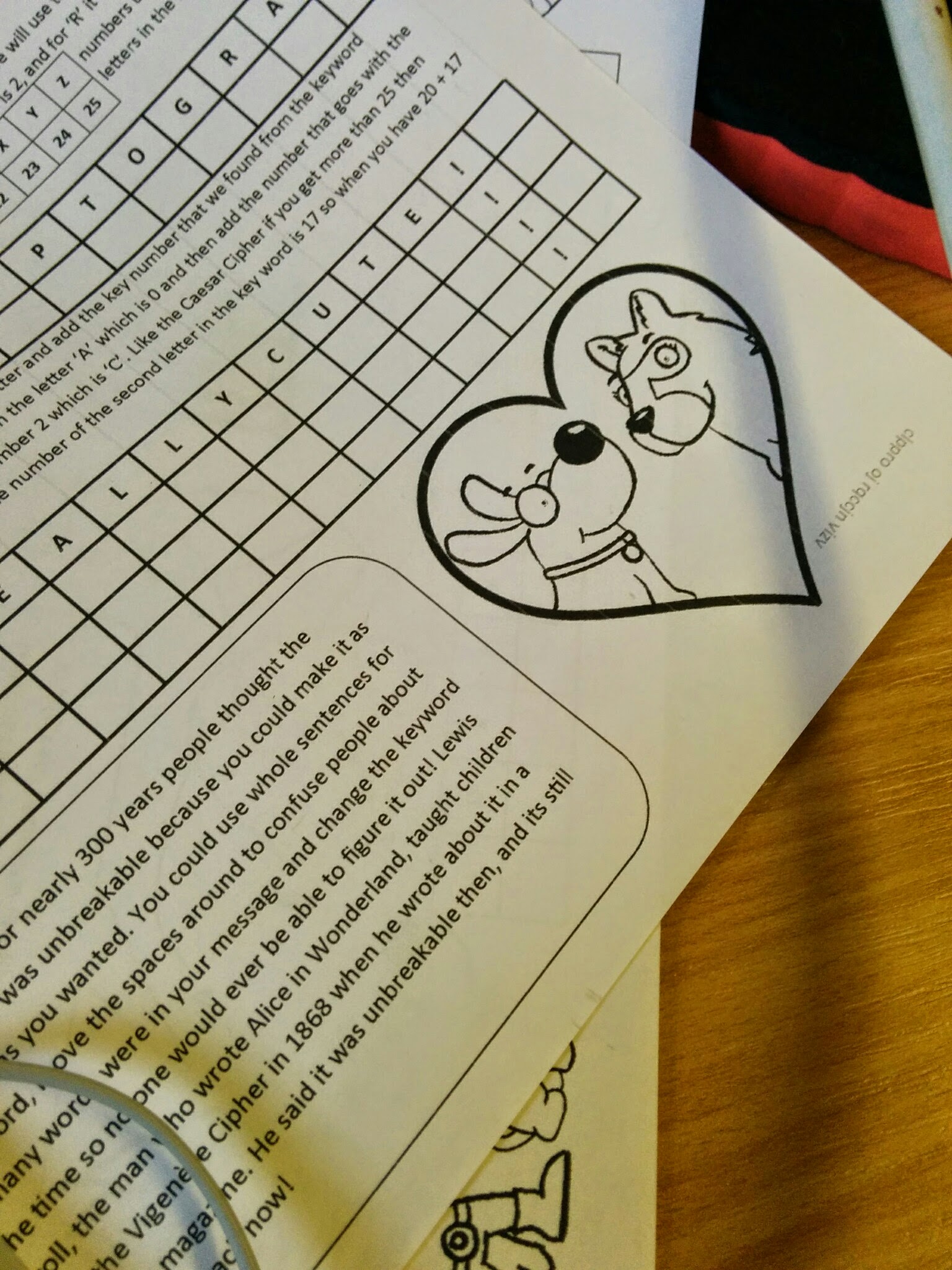
An outreach/educational package based around cryptography. They coded a variety of cyphers in Python and also put together an excellent set of teaching resources with really well drawn characters etc… They even threw in my dog Auraya (the likeness of the drawing is pretty awesome :)):
![]()
![]()
I ask my students to find an original way of showcasing their code. I don’t actually know the right answer to that ‘challenge’. Most students showcase the website and/or app, some will talk me through some code but this year one group did something quite frankly awesome: code on cake. Here’s some of the code they wrote for their phone app (written with kivy):
![]()
One group built a fully functioning and hosted web app (after taking a look at Django they decided that Flask was the way to go for this particular tool). Their app takes in a natural number and classifies it against a number of categories, go ahead and try it right now: Categorising Numbers
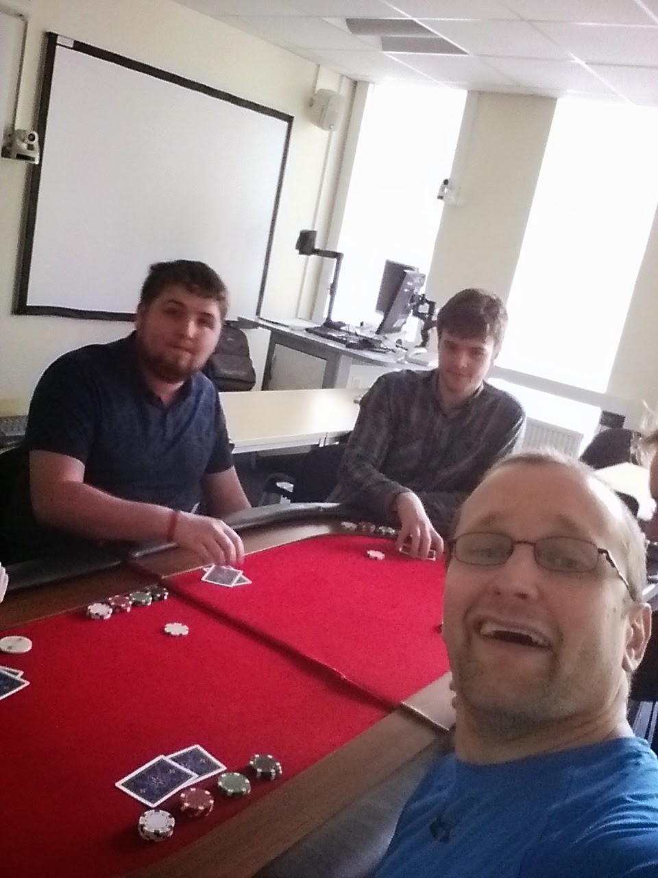
One of the more fun presentations was for a poker simulation app that uses a prime number representation of a hand of poker to simulate all possible outcomes of a given state. This work remarkably fast and immediately spits out (with neat graphics of the cards) the probability of winning given the current cards. As well as an impressive app the students presented it very well and invited me to play a game of poker (I lost, their mark was not affected…):
![]()
Here are a couple of screen shots of the app itself:
Home screen:
![]()
The input card screen:
![]()


I am missing out a bunch of great projects (including an impressive actual business that I will be delighted to talk about more when appropriate). I am very grateful to the efforts put in by all the students and wish them well during their exams.
↧
↧
Benjamin Hackl: Google Summer of Code — Countdown
Today I received the welcome package for attending this year’s “Google Summer of Code”! Actually, it’s pretty cool; the following things were included:
- a blue notebook with a monochromatic GSoC 15 logo (in dark blue) printed on it
- a sticker with a colored GSoC 15 logo
- a pen that is both a blue ballpoint pen as well as a mechanical pencil (0.5)
Here is a photo of all this stuff:

The work on our project (multivariate) Asymptotic Expressions (in cooperation with Daniel Krenn and Clemens Heuberger) begins (or rather continues) on Monday, the 25th of May. Over the course of next week (probably in a  -neighborhood of Monday) I will blog about the status quo, as well as about the motivation for the project.
↧
William Stein: Guiding principles for SageMath, Inc.
In February of this year (2015), I founded a Delaware C Corporation called "SageMath, Inc.". This is a first stab at the guiding principles for the company. It should help clarify the relationship between the company, the Sage project, and other projects like OpenDreamKit and Jupyter/IPython.
Company mission statement:
Make open source mathematical software ubiquitous.This involves both creating the SageMathCloud website and supporting the development and distribution of the SageMath and other software, including Jupyter, Octave, Scilab, etc. Anything open source.
Company principles:
- Absolutely all company funded software must be open source, under a GPLv3 compatible license. We are a 100% open source company.
- Company independence and self-determination is far more important than money. A core principle is that SMI is not for sale at any price, and will not participate in any partnership (for cost) that would restrict our freedom. This means:
- reject any offers from corp development from big companies to purchase or partner,
- do not take any investment money unless absolutely necessary, and then only from the highest quality investors
- do not take venture capital ever
- Be as open as possible about everything involving the company. What should not be open (since it is dangerous):
- security issues, passwords
- finances (which could attract trolls)
- private user data
- aggregate usage data, e.g., number of users.
- aggregate data that could help other open source projects improve their development, e.g., common problems we observe with Jupyter notebooks should be provided to their team.
- guiding principles
Business model
- SageMathCloud is freemium with the expectation that 2-5% of users pay.
- Target audience: all potential users of cloud-based math-related software.
SageMathCloud mission
Make it as easy as possible to use open source mathematical software in the cloud.This means:
- Minimize onboard friction, so in less than 1 minute, you can create an account and be using Sage or Jupyter or LaTeX. Morever, the UI should be simple and streamlined specifically for the tasks, while still having deep functionality to support expert users. Also, everything persists and can be sorted, searched, used later, etc.
- Minimize support friction, so one click from within SMC leads to a support forum, an easy way for admins to directly help, etc. This is not at all implemented yet. Also, a support marketplace where experts get paid to help non-experts (tutoring, etc.).
- Minimize teaching friction, so everything involving software related to teaching a course is as easy as possible, including managing a list of students, distributing and collecting homework, and automated grading and feedback.
- Minimize pay friction, sign up for a $7 monthly membership, then simple clear pay-as-you-go functionality if you need more power.
↧
Benjamin Hackl: Asymptotic Expressions: Motivation
So, as Google Summer of Code started on Monday, May 25th it is time to give a proper motivation for the project I have proposed. The working title of my project is (Multivariate) Asymptotic Expressions, and its overall goal is to bring asymptotic expressions to SageMath.
What are Asymptotic Expressions?
A motivating answer for this question comes from the theory of Taylor series. Assume that we have a sufficiently nice (in this case meaning smooth) function  that we want to approximate in a neighborhood of some point
  . Taylor’s theorem allows us to write
  where
where
![\[ T_n(x) = \sum_{j=0}^n \frac{f^{(j)}(x_0)}{j!}\cdot (x-x_0)^j = f(x_0) + f'(x_0)\cdot (x-x_0) + \cdots + \frac{f^{(n)}(x_0)}{n!}\cdot (x-x_0)^n, \]](http://benjamin-hackl.at/asdf-wp/wp-content/ql-cache/quicklatex.com-9c322e654df5f0f826ba652d1b743d2d_l3.png "Rendered by QuickLaTeX.com")
and  , where
  lies in a neighborhood of
  . Note that for
  ,
,  “behaves like”
  . In particular, we can certainly find a constant
  0" /> 0" title="Rendered by QuickLaTeX.com" height="12" width="47" style="vertical-align: 0px;" /> such that
  , or, in other words: for the growth of the function is bounded from above by the growth of .
The idea of bounding the growth of a function by the growth of another function when the argument approaches some number (or  ) is the central idea behind the big O notation. For function
  we write
  for if there is a constant 0" /> 0" title="Rendered by QuickLaTeX.com" height="12" width="47" style="vertical-align: 0px;" /> such that
  for all
  in some neighborhood of .
A case that is particularly important is the case of  , that is if we want to compare and/or characterize the behavior of some function for
  , which is also called the functions asymptotic behavior. For example, consider the functions
  ,
,  and
and  . All of them are growing unbounded for — however, their asymptotic behavior differs. This can be seen by considering pairwise quotients of these functions:
  for , and therefore the asymptotic growth of can be bounded above by the growth of , meaning
  for .
for .
The analysis of a functions asymptotic behavior is important for many applications, for example when determining time and space complexity of algorithms in computer science, or for describing the growth of classes of combinatorial objects: take, for example, binary strings of length  that contain equally many zeros and ones. If
  denotes the number of such strings, then we have
![\[ s_n = \binom{2n}{n} = \frac{4^n}{\sqrt{n\pi}} \left(1 + O\left(\frac{1}{n}\right)\right) \quad\text{ for } n\to\infty. \]](http://benjamin-hackl.at/asdf-wp/wp-content/ql-cache/quicklatex.com-f09413e7c95c203bfaaa0f54fd7fa83c_l3.png "Rendered by QuickLaTeX.com")
Expressions like these are asymptotic expressions. When we consider asymptotic expressions in only one variable, everything works out nicely as a total order is induced. But as soon as multiple variables are involved, we don’t have a total order any more. Consider, for example,  and
and  when and
  approach . These two elements cannot be compared to each other, which complicates computing with these expressions as they may contain multiple “irreducible” O-terms.
The following univariate and multivariate examples shall demonstrate how computing with such expressions looks like (all variables are assumed to go to ):
![\[ x + O(x) = O(x),\quad x^2 \cdot (x + O(1)) = x^3 + O(x^2),\quad O(x^2) \cdot O(x^3) = O(x^5), \]](http://benjamin-hackl.at/asdf-wp/wp-content/ql-cache/quicklatex.com-690ed4ebd933b86fb99f542d1bd83f3d_l3.png "Rendered by QuickLaTeX.com")
![\[ x y + O(x^2 y) = O(x^2y),\quad (y \log y + O(y)) (x^2 y + O(4^x \sqrt{x})) = x^2 y^2 \log y + O(x^2 y^2) + O(4^x \sqrt{x} y \log y). \]](http://benjamin-hackl.at/asdf-wp/wp-content/ql-cache/quicklatex.com-7d62b4942340f22047d7717cb66e4c85_l3.png "Rendered by QuickLaTeX.com")
Our plan is to provide an implementation based on which computations with these and more complicated expressions are possible.
Planned Structure
There are four core concepts of our implementation.
- Asymptotic Growth Groups: These are multiplicative groups that contain growth elements like
 ,
,  ,
,  . For starters, only univariate power growth groups will be implemented.
 ,
,  . For starters, only univariate power growth groups will be implemented.
- Asymptotic Term Monoids: These monoids contain asymptotic terms — in essence, these are summands of asymptotic terms. Apart from exact term monoids (growth elements with a coefficient), we will also implement O-term monoids as well as a term monoid for a deviation of O-terms. Asymptotic terms have (in addition to their group operation, multiplication) absorption as an additional operation: for example, O-terms are able to absorb all asymptotically “smaller” elements.
- Mutable Poset: As we have mentioned above, due to the fact that multivariate asymptotic expressions do not have a total order with respect to their growth, we need a partially ordered set (“Poset”) that deals with this structure such that operations like absorbing terms can be performed efficiently. The mutable poset is the central data structure that asymptotic expressions are built upon.
- Asymptotic Ring: This is our top-level structure which is also supposed to be the main interaction object for users. The asymptotic ring contains the asymptotic expressions, i.e. intelligently managed sums of asymptotic terms. All common operations shall be possible here. Furthermore, the interface should be intelligent enough such that admissible expressions from the symbolic ring can be directly converted into elements of the asymptotic ring.
Obviously, this “planned structure” is rather superficial. However, this is only to supplement the motivation for my project with some ideas on the implementation. I’ll go a lot more into the details of what I am currently implementing in the next few blog posts!
↧