1. simplicity and documentation: people have little time, and the faster they learn how to use the library, the better;
2. number of routines available;
3. speed: sometimes, the input is very big, and the algorithms take much time to finish, so that a fast implementation is fundamental.

Every year there is a big festival in Edinburgh called the fringe festival. I blogged about this a while ago, in that post I did a very basic bit of natural language processing aiming to try and identify what made things funny. In this blog post I’m going to push that a bit further by building a classification model that aims to predict if a joke is funny or not. (tldr: I don’t really succeed but but that’s mainly because I have very little data - having more data would not necessarily guarantee success either but the code and approach is what’s worth taking from this post… 😪).

If you want to skip the brief description and go straight to look at the code you can find the ipython notebook on github here and on cloud.sagemath here.

The data comes from a series of BBC articles which reports (more or less every year since 2011?) the top ten jokes at the fringe festival. This does in fact only give 60 odd jokes to work with…

Here is the latest winner (by Tim Vine):

I decided to sell my Hoover… well it was just collecting dust.

After cleaning it up slightly I’ve thrown that all in a json file here. So in order to import the data in to a panda data frame I just run:

importpandasdf=pandas.read_json('jokes.json')# Loading the json file

Pandas is great, I’ve been used to creating my own bespoke classes for handling data but in general just using pandas does the exact right job. At this point I basically follow along with this post on sentiment analysis of twitter which makes use of the ridiculously powerful nltk library.

We can use the nltk library to ‘tokenise’ and get rid of common words:

commonwords=[e.upper()foreinset(nltk.corpus.stopwords.words('english'))]# <- Need to download the corpus: import nltk; nltk.download()commonwords.extend(['M','VE'])# Adding a couple of things that need to be removedtokenizer=nltk.tokenize.RegexpTokenizer(r'\w+')# To be able to strip out unwanted things in stringsstring_to_list=lambdax:[el.upper()forelintokenizer.tokenize(x)ifel.upper()notincommonwords]df['Joke']=df['Raw_joke'].apply(string_to_list)

Note that this requires downloading one of the awesome corpuses (thats apparently the right way to say that) from nltk.

Here is how this looks:

joke='I decided to sell my Hoover... well it was just collecting dust.'string_to_list(joke)

which gives:

['DECIDED','SELL','HOOVER','WELL','COLLECTING','DUST']

We can now get started on building a classifier

Here is the general idea of what will be happening:

First of all we need to build up the ‘features’ of each joke, in other words pull the words out in to a nice easy format.

To do that we need to find all the words from our training data set, another way of describing this is that we need to build up our dictionary:

df['Year']=df['Year'].apply(int)defget_all_words(dataframe):"""    A function that gets all the words from the Joke column in a given dataframe"""all_words=[]forjkindataframe['Joke']:all_words.extend(jk)returnall_wordsall_words=get_all_words(df[df['Year']<=2013])# This uses all jokes before 2013 as our training data set.

We then build something that will tell us for each joke which of the overall words is in it:

defextract_features(joke,all_words):words=set(joke)features={}forwordinwords:features['contains(%s)'%word]=(wordinall_words)returnfeatures

Once we have done that, we just need to decide what we will call a funny joke. For this purpose We’ll use a funny_threshold and any joke that ranks above the funny_threshold in any given year will be considered funny:

funny_threshold=5df['Rank']=df['Rank'].apply(int)df['Funny']=df['Rank']<=funny_threshold

Now we just need to create a tuple for each joke that puts the features mentioned earlier and a classification (if the joke was funny or not) together:

df['Labeled_Feature']=zip(df['Features'],df['Funny'])

We can now (in one line of code!!!!) create a classifier:

classifier=nltk.NaiveBayesClassifier.train(df[df['Year']<=2013]['Labeled_Feature'])

This classifier will take into account all the words in a given joke and spit out if it’s funny or not. It can also give us some indication as to what makes a joke funny or not:

classifier.show_most_informative_features(10)

Here is the output of that:

MostInformativeFeaturescontains(GOT)=TrueFalse:True=2.4:1.0contains(KNOW)=TrueTrue:False=1.7:1.0contains(PEOPLE)=TrueFalse:True=1.7:1.0contains(SEX)=TrueFalse:True=1.7:1.0contains(NEVER)=TrueFalse:True=1.7:1.0contains(RE)=TrueTrue:False=1.6:1.0contains(FRIEND)=TrueTrue:False=1.6:1.0contains(SAY)=TrueTrue:False=1.6:1.0contains(BOUGHT)=TrueTrue:False=1.6:1.0contains(ONE)=TrueTrue:False=1.5:1.0

This immediately gives us some information:

• If your joke is about SEX is it more likely to not be funny.
• If your joke is about FRIENDs is it more likely to be funny.

That’s all very nice but we can now (theoretically - again, I really don’t have enough data for this) start using the mathematical model to tell you if something is funny:

joke='Why was 10 afraid of 7? Because 7 8 9'classifier.classify(extract_features(string_to_list(joke),get_all_words(df[df['Year']<=2013])))

That joke is apparently funny (the output of above is True). The following joke however is apparently not (the output of below if False):

joke='Your mother is ...'printclassifier.classify(extract_features(string_to_list(joke),get_all_words(df[df['Year']<=2013])))

As you can see in the ipython notebook it is then very easy to measure how good the predictions are (I used the data from years before 2013 to predict 2014).

Results

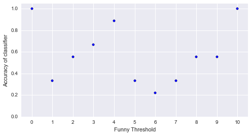
Here is a plot of the accuracy of the classifier for changing values of funny_threshold:

You’ll notice a couple of things:

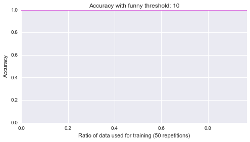
• When the threshold is 0 or 1: the classifier works perfectly. This makes sense: all the jokes are either funny or not so it’s very easy for the classifier to do well.
• There seems to be a couple of regions where the classifier does particularly poorly: just after a value of 4. Indeed there are points where the classifier does worse than flipping a coin.
• At a value of 4, the classifier does particularly well!

Now, one final thing I’ll take a look at is what happens if I start randomly selecting a portion of the entire data set to be the training set:

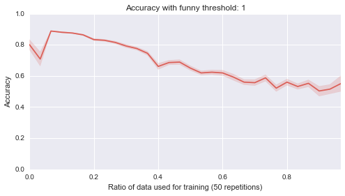
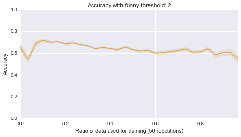
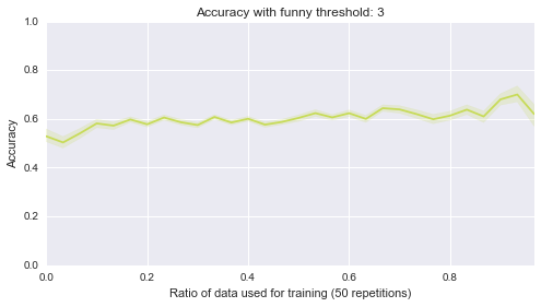
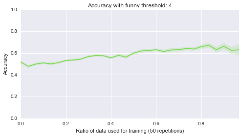
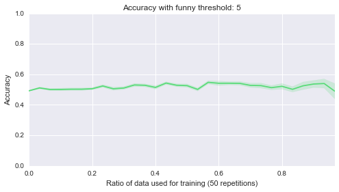
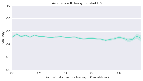
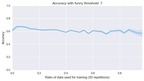
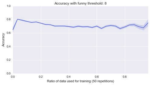
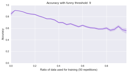
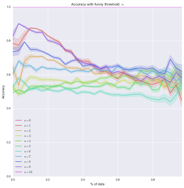
Below are 10 plots that correspond to 50 repetitions of the above where I randomly sample a ratio of the data set to be the training set:

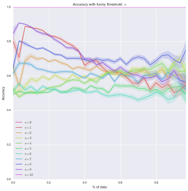
Finally (although it’s really not helpful), here are all of those on a single plot:

First of all: all those plots are basically one line of seaborn code which is ridiculously cool. Seaborn is basically magic:

sns.tsplot(data,steps)

Second of all, it looks like the lower bound of the classifiers is around .5. Most of them start of at .5, in other words they are as good as flipping a coin before we let them learn from anything, which makes sense. Finally it seems that the threshold of 4 classifier seems to be the only one that gradually improves as more data is given to it. That’s perhaps indicating that something interesting is happening there but that investigation would be for another day.

All of the conclusions about the actual data should certainly not be taken seriously: I simply do not have enough data. But, the overall process and code is what is worth taking away. It’s pretty neat that the variety of awesome python libraries lets you do this sort of thing more or less out of the box.

Please do take a look at this github repository but I’ve also just put the notebook on cloud.sagemath so assuming you pip install the libraries and get the data etc you can play around with this right in your browser:

Here is the notebook on cloud.sagemath.

We (James Campbell and Vince Knight are writing this together) have been working on implementing code in Sage to test if a game is degenerate or not. In this post we’ll prove a simple result that is used in the algorithm that we are/have implemented.

Bi-Matrix games

For a general overview of these sorts of things take a look at this post from a while ago on the subject of bi-matrix games in Sage. A bi-matrix is a matrix of tuples corresponding to payoffs for a 2 player Normal Form Game. Rows represent strategies for the first player and columns represent strategies for the second player, and each tuple of the bi-matrix corresponds to a tuple of payoffs. Here is an example:

We see that if the first player plays their third row strategy and the second player their second column strategy then the first player gets a utility of 6 and the second player a utility of 1.

This can also be written as two separate matrices. A matrix \(A\) for Player 1 and \(B\) for Player 2.

Here is how this can be constructed in Sage using the NormalFormGame class:

sage:A=matrix([[3,3],[2,5],[0,6]])sage:B=matrix([[3,2],[2,6],[3,1]])sage:g=NormalFormGame([A,B])sage:gNormalFormGamewiththefollowingutilities:{(0,1):[3,2],(0,0):[3,3],(2,1):[6,1],(2,0):[0,3],(1,0):[2,2],(1,1):[5,6]}

Currently, within Sage, we can obtain the Nash equilibria of games:

sage:g.obtain_nash()[[(0,1/3,2/3),(1/3,2/3)],[(4/5,1/5,0),(2/3,1/3)],[(1,0,0),(1,0)]]

We see that this game has 3 Nash equilibria. For each, we see that the supports (the number of non zero entries) of both players’ strategies are the same size. This is, in fact, a theoretical certainty when games are non degenerate.

If we modify the game slightly:

sage:A=matrix([[3,3],[2,5],[0,6]])sage:B=matrix([[3,3],[2,6],[3,1]])sage:g=NormalFormGame([A,B])sage:g.obtain_nash()[[(0,1/3,2/3),(1/3,2/3)],[(1,0,0),(2/3,1/3)],[(1,0,0),(1,0)]]

We see that the second equilibrium has supports of different sizes. In fact, if the first player did play \((1,0,0)\) (in other words just play the first row) the second player could play any mixture of strategies as a best response and not particularly \((2/3,1/3)\). This is because the game in consideration is now degenerate.

(Note that both of the games above are taken from Nisan et al. 2007 [pdf].)

What is a degenerate game

A bimatrix game is called nondegenerate if the number of pure best responses to a mixed strategy never exceeds the size of its support. In a degenerate game, this definition is violated, for example if there is a pure strategy that has two pure best responses (as in the example above), but it is also possible to have a mixed strategy with support size \(k\) that has \(k+1\) strategies that are a best response.

Here is an example of this:

If we consider the mixed strategy for player 2: \(y=(1/2,1/2)\), then the utility to player 1 is given by:

We see that there are 3 best responses to \(y\) and as \(y\) has support size 2 this implies that the game above is degenerate.

What does the literature say about degenerate games

The original definition of degenerate games was given in Lemke, Howson 1964 [pdf] and their definition was dependent on the labeling polytope that they used for their famous algorithm for the computation of equilibria (which is currently being implemented in Sage!). Further to this Stengel 1999 [ps] offers a nice overview of a variety of equivalent definitions.

Sadly, all of these definitions require finding a particular mixed strategy profile \((x, y)\) for which a particular condition holds. To be able to implement a test for degeneracy based on any of these definitions would require a continuous search over possible mixed strategy pairs.

In the previous example (where we take \(y=(1/2,1/2)\) we could have identified this \(y\) by looking at the utilities for each pure strategy for player 1 against \(y=(y_1, 1-y_1)\):

(\(r_i\) denotes row strategy \(i\) for player 1.) A plot of this is shown:

We can (in this instance) quickly search through values of \(y_1\) and identify the point that has the most best responses which gives the best chance of passing the degeneracy condition (\(y_1=1/2\)). This is not really practical from a generic point of view which leads to this blog post: we have identified what the particular \(x, y\) is that is sufficient to test.

A sufficient mixed strategy to test for degeneracy

The definition of degeneracy can be written as:

Def. A Normal Form Game is degenerate iff:

There exists \(x\in \Delta X\) such that \( |S(x)| < |\sigma_2| \) where \(\sigma_2\) is the support such that \( (xB)_j = \max(xB) \), for all \(j \) in \( \sigma_2\).

OR

There exists \(y\in \Delta Y\) such that \( |S(x)| < |\sigma_1| \) where \(\sigma_1\) is the support such that \( (Ay)_i = \max(Ay) \), for all \(i \) in \( \sigma_1\).

(\(X\) and \(Y\) are the pure strategies for player 1 and 2 and \(\Delta X, \Delta Y\) the corresponding mixed strategies spaces.

The result we are implementing in Sage aims to remove the need to search particular mixed strategies \(x, y\) (a continuous search) and replace that by a search over supports (a discrete search).

Theorem. A Normal Form Game is degenerate iff:

There exists \( \sigma_1 \subseteq X \) and \( \sigma_2 \subseteq Y \) such that \( |\sigma_1| < |\sigma_2| \) and \( S(x^*) = \sigma_1 \) where \( x^* \) is a solution of \( (xB)_j = \max(xB) \), for all \(j \) in \( \sigma_2 \) (note that a valid \(x^*\) is understood to be a mixed strategy vector).

OR

There exists \( \sigma_1 \subseteq X \) and \( \sigma_2 \subseteq Y \) such that \( |\sigma_1| > |\sigma_2| \) and \( S(y^*) = \sigma_2 \) where \( y^* \) is a solution of \( (Ay)_i = \max(Ay) \), for all \(i \) in \( \sigma_1 \).

Using the definition given above the proof is relatively straightforward but we will include it below (mainly to try and convince ourselves that we haven’t made a mistake).

We will only consider the first part of each condition (the ones for the first player). The result follows in the same way for the second player.

Proof \(\Leftarrow\)

Assume a game defined by \(A, B\) is degenerate, by the above definition without loss of generality this implies that there exists an \(x\in \Delta X\) such that \( |S(x)| < |\sigma_2| \) where \(\sigma_2\) is the support such that \( (xB)_j = \max(xB) \), for all \(j \) in \( \sigma_2\).

If we denote \(S(x)\) by \(\sigma_1\) then the definition implies that \(|\sigma_1| < |\sigma_2| \) and further more that \( (xB)_j = \max(xB) \), for all \(j \) in \( \sigma_2 \) as required.

Proof \(\Rightarrow\)

If we now assume that we have \(\sigma_1, \sigma_2, x^*\) as per the first part of the theorem then we have \(|\sigma_1|<|\sigma_2|\) and taking \(x=x^*\) implies that \(|S(x)|<|\sigma_2|\). Furthermore as \(x^*\) is a solution of \( (xB)_j = \max(xB) \) the result follows (by the definition given above).

Implementation

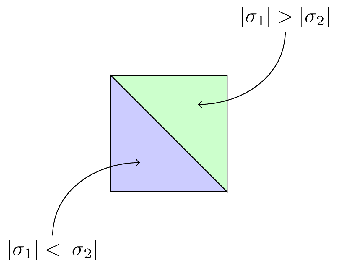
This result implies that we simply need to consider all potential pairs of supports. Depending on the relative size of the supports we can use one of the two conditions of the result. If we ordered the supports by size the situation for the two player game looks somewhat like this:

Note that for an \(m\times n\) game there are \((2^m-1)\) potential supports for player 1 (the size of the powerset of strategy set without the empty set) and \((2^n-1)\) potential supports of for player 2. Thus the rectangle drawn above has dimension \((2^m-1)\times(2^n-1)\). Needless to say that our implementation will not be efficient (testing degeneracy is after all an NP complete problem in linear programming (see Chandrasekaran 1982 - [pdf]) but at least we have identified exactly which mixed strategy we need to test for each support pair.

References

• Chandrasekaran, R., Santosh N. Kabadi, and Katta G. Murthy. “Some NP-complete problems in linear programming.” Operations Research Letters 1.3 (1982): 101-104. [pdf]
• Lemke, Carlton E., and Joseph T. Howson, Jr. “Equilibrium points of bimatrix games.” Journal of the Society for Industrial & Applied Mathematics 12.2 (1964): 413-423. [pdf]
• N Nisan, T Roughgarden, E Tardos, VV Vazirani Vol. 1. Cambridge: Cambridge University Press, 2007. [pdf]
• von Stengel, B. “Computing equilibria for two person games.” Technical report. [ps]

Clustering Coefficient

Dominator tree

Cuthill-McKee ordering / King ordering

Dijkstra/Bellman-Ford/Johnson shortest paths

It has been quite some time since my last update on the progress of my Google Summer of Code project, which has two reasons. On the one hand, I have been busy because of the end of the semester, as well as because of the finalization of my Master’s thesis — and on the other hand, it is not very interesting to write a post on discussing and implementing rather technical details. Nevertheless, Daniel Krenn and myself have been quite busy in order to bring asymptotic expressions to SageMath. Fortunately, these efforts are starting to become quite fruitful.

In this post I want to discuss our current implementation roadmap (i.e. not only for the remaining Summer of Code, but also for the time afterwards), and give some examples for what we are currently able to do.

Strutcture and Roadmap

An overview of the entire roadmap can be found at here (trac #17601). Recall that the overall goal of this project is to bring asymptotic expressions like $2^n + n^2 \log n + O(n)$ to Sage. Our implementation (which aims to be as general and expandable as possible) tackles this problem with a three-layer approach:

• GrowthGroups and GrowthElements (trac #17600). These elements and parents manage the growth (and just the growth!) of a summand in an asymptotic expression like above. The simplest cases are monomial and logarithmic growth groups. For example, their elements are given by $n^r$ and $\log(n)^r$ where the exponent $r$ is from some ordered ring like $\mathbb{Z}$ or $\mathbb{Q}$. Both cases (monomial and logarithmic growth groups) can be handled in the current implementation — however, growth elements like $n^2 \log n$ are intended to live in the cartesian product of a monomial and a logarithmic growth group (in the same variable). Parts of this infrastructure are already prepared (see trac #18587).
• AsymptoticTerms and TermMonoids (trac #17715). While GrowthElements only represent the growth, AsymptoticTerms have more information: basically, they represent a summand in an asymptotic expression. There are different classes for each type of asymptotic term (e.g. ExactTerm and OTerm — with more to come). Additionally to a growth element, some types of asymptotic terms (like exact terms) also possess a coefficient.
• AsymptoticExpression and AsymptoticRing (trac #17716). This is what we are currently working on, and we do have a running prototype! The version that can be found on trac is only missing some doctests and a bit of documentation. Asymptotic expressions are the central objects within this project, and essentially they are sums of several asymptotic terms. In the background, we use a special data structure (“mutable posets“, trac #17693) in order to model the (partial) order induced by the various growth elements belonging to an asymptotic expression. This allows to perform critical operations like absorption (when an \(O\)-term absorbs “weaker” terms) efficiently and in a simple way.

The resulting minimal prototype can, in some sense, be compared to Sage’s PowerSeriesRing: however, we also allow non-integer coefficients, and extending this prototype to work with multivariate expressions should not be too hard now, as the necessary infrastructure is there.

Following the finalization of the minimal prototype, there are several improvements to be made. Here are some examples:

• Besides addition and multiplication, we also want to divide asymptotic expressions, and higher-order operations like exponentiation and taking the logarithm would be interesting as well.
• Also, conversion from, for example, the symbolic ring is important when it comes to usability of our tools. We will implement and enhance this conversion gradually.

Examples

An asymptotic ring (over a monomial growth group with coefficients and exponents from the rational field) can be created with

sage: R.<x> = AsymptoticRing('monomial', QQ); R
Asymptotic Ring over Monomial Growth Group in x over Rational Field with coefficients from Rational Field

Note that we marked the code as experimental, meaning that you will see some warnings regarding the stability of the code. Now, as we have an asymptotic ring, we can do some calculations. For example, take $ (2\sqrt{x} + O(1))^{15}$:

sage: (2*x^(1/2) + O(x^0))^15
O(x^7) + 32768*x^(15/2)

We can also have a look at the underlying structure:

sage: expr = (x^(3/7) + 2*x^(1/5)) * (x + O(x^0)); expr
O(x^(3/7)) + 2*x^(6/5) + 1*x^(10/7)
sage: expr.poset
poset(O(x^(3/7)), 2*x^(6/5), 1*x^(10/7))
sage: print expr.poset.full_repr()
poset(O(x^(3/7)), 2*x^(6/5), 1*x^(10/7))
+-- null
|   +-- no predecessors
|   +-- successors:   O(x^(3/7))
+-- O(x^(3/7))
|   +-- predecessors:   null
|   +-- successors:   2*x^(6/5)
+-- 2*x^(6/5)
|   +-- predecessors:   O(x^(3/7))
|   +-- successors:   1*x^(10/7)
+-- 1*x^(10/7)
|   +-- predecessors:   2*x^(6/5)
|   +-- successors:   oo
+-- oo
|   +-- predecessors:   1*x^(10/7)
|   +-- no successors

As you might have noticed, the “O”-constructor that is used for the PowerSeriesRing and related structures, can also be used here. In particular, $O(\mathit{expr})$ acts exactly as expected:

sage: expr
O(x^(3/7)) + 2*x^(6/5) + 1*x^(10/7)
sage: O(expr)
O(x^(10/7))

Of course, the usual rules for computing with asymptotic expressions hold:

sage: O(x) + O(x)
O(x)
sage: O(x) - O(x)
O(x)

So far, so good. Our next step is making the multivariate growth groups usable for the AsymptoticRing and then improving the overall user interface of the ring.

This past week I have been delighted to have a short pedagogic paper accepted for publication in MSOR Connections. The paper is entitled: “Playing Games: A Case Study in Active Learning Applied to Game Theory”. The journal is open access and you can see a pre print here. As well as describing some literature on active learning I also present some data I’ve been collecting (with the help of others) as to how people play two subsequent plays of the two thirds of the average game (and talk about another game also).

In this post I’ll briefly put up the results here as well as mention a Python library I’m working on.

If you’re not familiar with it, the two thirds of the average game asks players to guess a number between 0 and 100. The closest number to 2/3rds of the average number guessed is declared the winner.

I use this all the time in class and during outreach events. I start by asking participants to play without more explanation than the basic rules of the game. Following this, as a group we go over some simple best response dynamics that indicate that the equilibrium play for the game is for everyone to guess 0. After this explanation, everyone plays again.

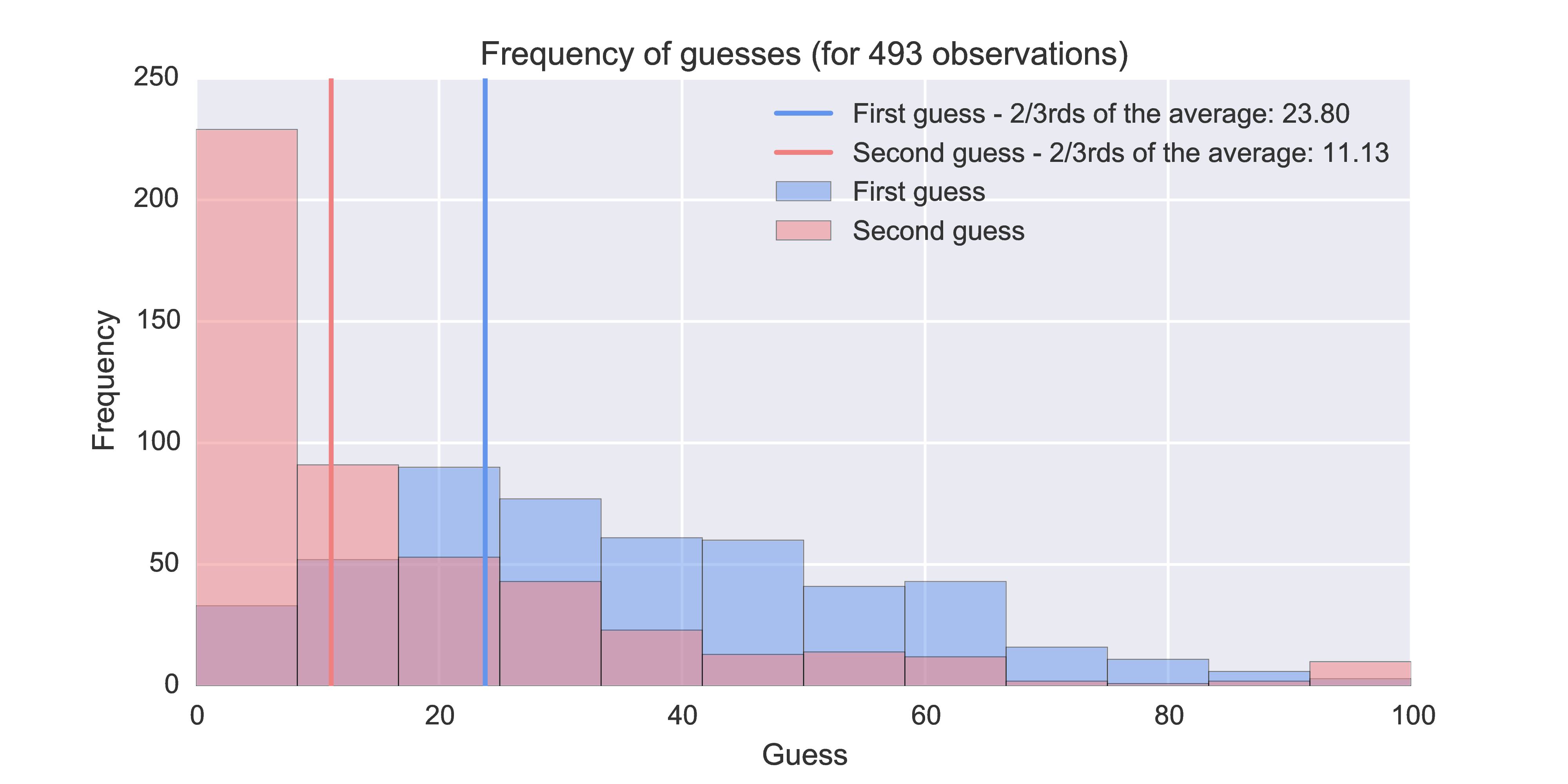
Below you can see how this game has gone as a collection of all the data I’ve put together:

You will note that some participants actually increase their second guess but in general we see a possible indication (based on two data points, so obviously this is not meant to be a conclusive statement) of convergence towards the theoretic equilibria.

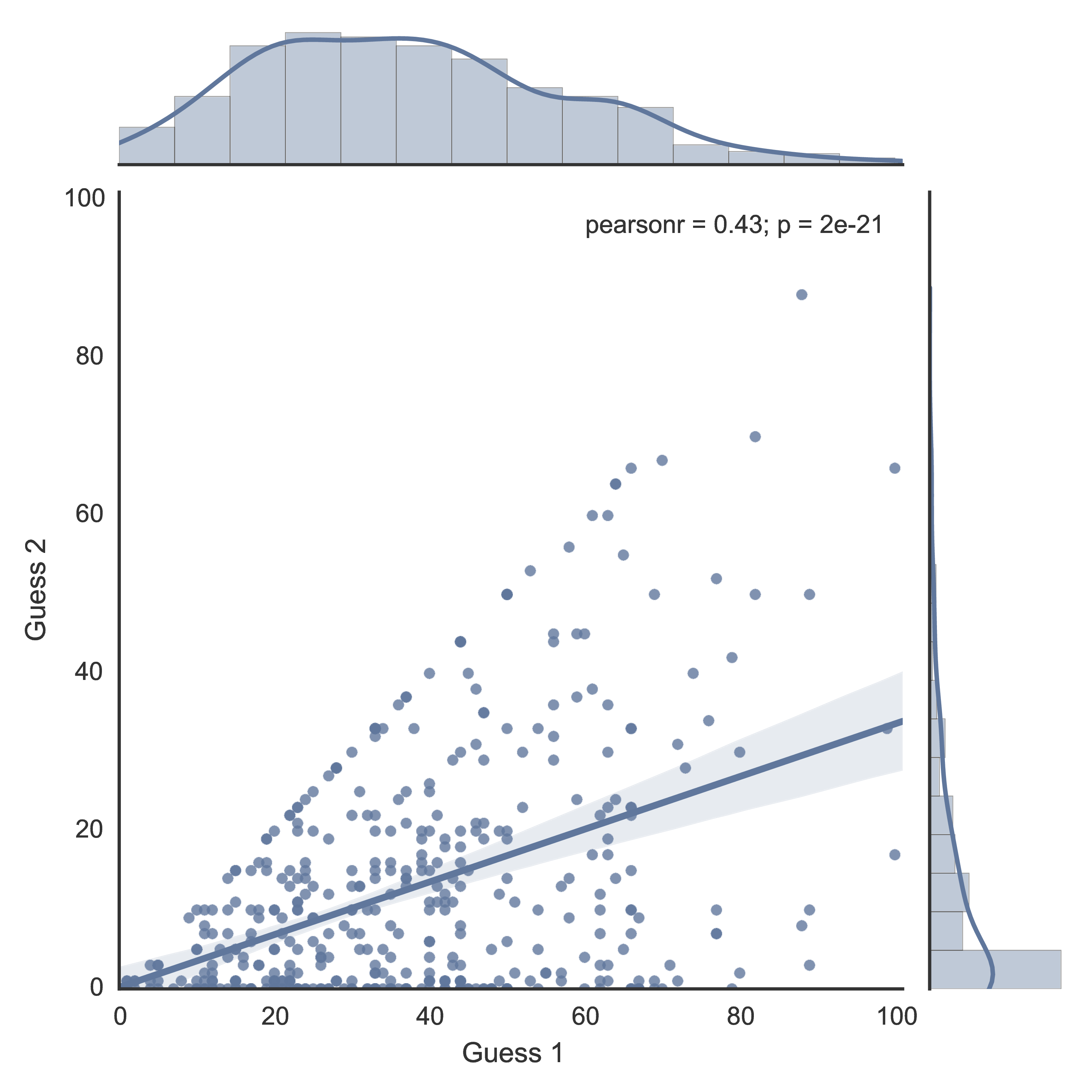
Here is a plot showing the relationship between the first and second guess (when removing the guesses that increase, although as you can see in the paper this does not make much difference):

The significant linear relationship between the guesses is given by:

So a good indication of what someone will guess in the second round is that it would be a third of their first round guess.

Here is some Sage code that produces the cobweb diagram assuming the following sequence represents each guess (using code by Marshall Hampton):

that plot shows the iterations of the hypothetical guesses if we were to play more rounds :)

The other thing I wanted to point at in this blog post is this twothirds library which will potentially allow anyone to analyse these games quickly. I’m still working on it but if it’s of interest please do jump in :) I have put up a Jupyter notebook demoing what it can do so far (which is almost everything but with some rough edges). If you want to try it out, download that notebook and run:

$ pip install twothirds

I hope that once the library is set up anyone who uses it could simply send over data of game plays via PR which would help update the above plots and conclusions :)

Today, Cardiff University, School of Mathematics students: James Campbell, Hannah Lorrimore as well as Google Summer of Code student Tobenna P. Igwe (PhD student at the University of Liverpool) as well as I presented the current game theoretic capabilities of Sagemath.

This talk happened as part of a two day visit to see Dima Pasechnik to work on the stuff we’ve been doing and the visit was kindly supported by CoDiMa (an EPSRC funded project to support the development of GAP and Sagemath)

Here is the video of the talk:

Here is a link to the sage worksheet we used for the talk.

Here are some photos I took during the talk:

and here are some I took of us working on code afterwards:

Here is the abstract of the talk:

Game Theory is the study of rational interaction and is getting increasingly important in CS. Ability to quickly compute a solution concept for a nontrivial (non-)cooperative game helps a lot in practical and theoretic work, as well as in teaching. This talk will describe and demonstrate the game theoretic capabilities of Sagemath (http://www.sagemath.org/), a Python library, described as having the following mission: ‘Creating a viable free opensource alternative to Magma, Maple, Mathematica and Matlab’.

The talk will describe algorithms and classes that are implemented for the computation of Nash equilibria in bimatrix games. These include:

• A support enumeration algorithm;
• A reverse search algorithm through the lrs library;
• The Lemke-Howson algorithm using the Gambit library (https://github.com/gambitproject/gambit).

In addition to this, demonstrations of further capabilities that are actively being developed will also be given:

• Tests for degeneracy in games;
• A class for extensive form games which include the use of the graph theoretic capabilities of Sage.

The following two developments which are being carried out as part of a Google Summer of Code project will also be demonstrated:

• An implementation of the Lemke-Howson algorithm;
• Extensions to N player games;

Demonstrations will use the (free) online tool cloud.sagemath which allows anyone with connectivity to use Sage (and solve game theoretic problems!). Cloud.sagemath also serves as a great teaching and research tool with access to not only Sage but Jupyter (Ipython) notebooks, R, LaTeX and a variety of other software tools.

The talk will concentrate on strategic non-cooperative games but matching games and characteristic function games will also be briefly discussed.

In a blog post I wrote in 2013, I showed how to simulate a discrete Markov chain. In this post we’ll (written with a bit of help from Geraint Palmer) show how to do the same with a continuous chain which can be used to speedily obtain steady state distributions for models of queueing processes for example.

A continuous Markov chain is defined by a transition rate matrix which shows the rates at which transitions from 1 state to an other occur. Here is an example of a continuous Markov chain:

This has transition rate matrix \(Q\) given by:

The diagonals have negative entries, which can be interpreted as a rate of no change. To obtain the steady state probabilities \(\pi\) for this chain we can solve the following matrix equation:

if we include the fact that the sum of \(\pi\) must be 1 (so that it is indeed a probability vector) we can obtain the probabilities in Sagemath using the following:

You can run this here (just click on ‘Evaluate’):

Q=matrix(QQ,[[-3,2,1],[1,-5,4],[1,8,-9]])(transpose(Q).stack(vector([1,1,1])).solve_right(vector([0,0,0,1])))

This returns:

(1/4,1/2,1/4)

Thus, if we were to randomly observe this chain:

• 25% of the time it would be in state 1;
• 50% of the time it would be in state 2;
• 25% of the time it would be in state 3.

Now, the markov chain in question means that if we’re in the first state the rate at which a change happens to go to the second state is 2 and the rate at which a change happens that goes to the third state is 1.

This is analagous to waiting at a bus stop at the first city. Buses to the second city arrive randomly 2 per hour, and buses to the third city arrive randomly 1 per hour. Everyone waiting for a bus catches the first one that arrives. So at steady state the population will be spread amongst the three cities according to \(\pi\).

Consider yourself at this bus stop. As all this is Markovian we do not care what time you arrived at the bus stop (memoryless property). You expect the bus to the second city to arrive 1/2 hours from now, with randomness, and the bus to the third city to arrive 1 hour from now, with randomness.

To simulate this we can sample two random numbers from the exponential distribution and find out which bus arrives first and ‘catch that bus’:

importrandom[random.expovariate(2),random.expovariate(1)]

The above returned (for this particular instance):

[0.5003491524841699,0.6107995795458322]

So here it’s going to take .5 hours for a bus to the second city to arrive, whereas it would take .61 hours for a bus to the third. So we would catch the bust to the second city after spending 0.5 hours at the first city.

We can use this to write a function that will take a transition rate matrix, simulate the transitions and keep track of the time spent in each state:

defsample_from_rate(rate):importrandomifrate==0:returnooreturnrandom.expovariate(rate)defsimulate_cmc(Q,time,warm_up):Q=list(Q)# In case a matrix is inputstate_space=range(len(Q))# Index the state spacetime_spent={s:0forsinstate_space}# Set up a dictionary to keep track of timeclock=0# Keep track of the clockcurrent_state=0# First statewhileclock<time:# Sample the transitionssojourn_times=[sample_from_rate(rate)forrateinQ[current_state][:current_state]]sojourn_times+=[oo]# An infinite sojourn to the same statesojourn_times+=[sample_from_rate(rate)forrateinQ[current_state][current_state+1:]]# Identify the next statenext_state=min(state_space,key=lambdax:sojourn_times[x])sojourn=sojourn_times[next_state]clock+=sojournifclock>warm_up:# Keep track if past warm up timetime_spent[current_state]+=sojourncurrent_state=next_state# Transitionpi=[time_spent[state]/sum(time_spent.values())forstateinstate_space]# Calculate probabilitiesreturnpi

Here are the probabilities from the same Markov chain as above:

which gave (on one particular run):

[0.25447326473556037,0.49567517998307603,0.24985155528136352]

This approach was used by Geraint Palmer who is doing a PhD with Paul Harper and I. He used this to verify that calculations were being carried out correctly when he was trying to fit a model. James Campbell and I are going to try to use this to get an approximation for bigger chains that cannot be solved analytically in a reasonable amount of time. In essence the simulation of the Markov chain makes sure we spend time calculating probabilities in states that are common.

If you are not familiar with Sagemath it is a free open source mathematics package that does simple things like expand algebraic expressions as well as far more complex things (optimisation, graph theory, combinatorics, game theory etc…). Cloud.sagemath is a truly amazing tool not just for Sage bu for scientific computation in general and it’s free. Completely 100% free. In this post I’ll explain why I pay for it.

A while ago, a colleague and I were having a chat about the fact that our site Maple license hadn’t been renewed fast enough (or something similar to that). My colleague was fairly annoyed by this saying something like:

‘We are kind of like professional athletes, if I played soccer at a professional club I would have the best facilities available to me. There would not be a question of me having the best boots.’

Now I don’t think we ever finished this conversation (or at least I don’t really remember what I said) but this is something that’s stayed with me for quite a while.

First of all:

I think there are probably a very large proportion of professional soccer players who do not play at the very top level and so do not enjoy having access to the very best facilities (I certainly wouldn’t consider myself the Ronaldo of mathematics…).

Secondly:

Mathematicians are (in some ways) way cooler than soccer players. We are somewhat like magicians, in the past we have not needed much more than a pencil and some paper to work our craft. Whilst a chemist/physicist/medical research needs a lab and/or other things we can pretty much work just with a whiteboard.

We are basically magicians. We can make something from nothing.

Since moving to open source software for all my research and teaching this is certainly how I’ve felt. Before discovering open source tools I needed to make sure I had the correct licence or otherwise before I could work but this is no longer the case. I just need a very basic computer (I bought a thinkpad for £60 the other day!) and I am just as powerful as I could want to be.

This is even more true with cloud.sagemath. Anyone can use a variety of scientific computing tools for no cost whatsoever (not even a cost associated with the time spent installing software): it just works. I have used this to work on sage source code with students, carry out research and also to deliver presentations: it’s awesome.

So, why do I pay $7 month to use it?

Firstly because it gives me the ability to move some projects to servers that are supposedly more robust. I have no doubt that they are more robust but in all honesty I can’t say I’ve seen problems with the ‘less’ robust servers (150 of my students used them last year and will be doing so again in the Autumn).

The main reason I pay to use cloud.sagemath is because I can afford to.

This was put in very clear terms to me during the organisation of DjangoCon Europe. The principle at Python conferences is that everyone pays to attend. This in turn ensures that funds are available for people who cannot afford to pay to attend.

I am in a lucky enough financial position that for about the price of two fancy cups of coffee a month I can help support an absolutely amazing project that helps everyone and anyone have the same powers a magician does. This helps (although my contribution is obviously a very small part of it) ensure that students and anyone else who cannot afford to help support the project, can use Sage.

• Edge connectivity (trac.sagemath.org/ticket/18564);
• Clustering coefficient (trac.sagemath.org/ticket/18811);
• Cuthill-McKee and King vertex orderings (trac.sagemath.org/ticket/18876);
• Minimum spanning tree(trac.sagemath.org/ticket/18910);
• Dijkstra, Bellman-Ford, Johnson shortest paths(trac.sagemath.org/ticket/18931);

Since my last blog entry on the status of our implementation of Asymptotic Expressions in SageMath quite a lot of improvements have happened. Essentially, all the pieces required in order to have a basic working implementation of multivariate asymptotics are there. The remaining tasks within my Google Summer of Code project are:

• Polish the documentation of our minimal prototype, which consists of #17716 and the respective dependencies. Afterwards, we will set this to needs_review.
• Open a ticket for the multivariate asymptotic ring and put together everything that we have written so far there.

In this blog post I want to give some more examples of what can be done with our implementation right now and what we would like to be able to handle in the future.

Status Quo

After I wrote my last blog entry, we introduced a central idea/interface to our project: short notations. By using the short notation factory for growth groups (introduced in #18930) it becomes very simple to construct the desired growth group. Essentially, monomial growth groups (cf. #17600), i.e. groups that contain elements of the form

variable^power

variable^base

sage: from sage.groups.asymptotic_growth_group import GrowthGroup
sage: G = GrowthGroup('x^ZZ'); G
Growth Group x^ZZ
sage: G.an_element()
x
sage: G = GrowthGroup('x^QQ'); G
Growth Group x^QQ
sage: G.an_element()
x^(1/2)

Naturally, this interface carries over to the generation of asymptotic rings: instead of the (slightly dubious)

"monomial"

sage: R.<x> = AsymptoticRing('x^ZZ', QQ); R
Asymptotic Ring <x^ZZ> over Rational Field
sage: (x^2 + O(x))^50
x^100 + O(x^99)

Recently, we also implemented another type of growth group: exponential growth groups (see #19028). These groups represent elements of the form

base^variable

sage: G = GrowthGroup('QQ^x'); G
Growth Group QQ^x
sage: G.an_element()
(1/2)^x
sage: G(2^x) * G(3^x)
6^x
sage: G(5^x) * G((1/7)^x)
(5/7)^x

Note: unfortunately, we did not implement a function that allows taking some element from some growth group (e.g.

x

We also made this short notation a central interface for working with cartesian products. This is implemented in #18587. For example, this allows to construct growth groups containing elements like $2^x \sqrt[5]{x^2} \log(x)^2$:

sage: G = GrowthGroup('QQ^x * x^QQ * log(x)^ZZ'); G
Growth Group QQ^x * x^QQ * log(x)^ZZ
sage: G.an_element()
(1/2)^x * x^(1/2) * log(x)
sage: G(2^x * x^(2/5) * log(x)^2)
2^x * x^(2/5) * log(x)^2

Simple parsing from the symbolic ring (and from strings) is implemented. Like I have written above, operations like

2^G(x)

log(G(x))

Further Steps

Of course, having an easy way to generate growth groups (and thus also asymptotic rings) is nice — however, it would be even better if the process of finding the correct parent would be even more automated. Unfortunately, this requires some non-trivial effort regarding the pushout construction — which will certainly not happen within the GSoC project.

As soon as we have an efficient way to “switch” between factors of a growth group (e.g. by taking the logarithm or the exponential function), this has to be carried over up to the asymptotic ring. Operations like

sage: 2^(x^2 + O(x))
2^(x^2) * 2^(O(x))

where the output could also be

2^(x^2) * O(x^g)

series_precision()

Division of asymptotic expressions can be realized with just about the same idea, for example:

\[ \frac{1}{x^2 + O(x)} = \frac{1}{x^2} \frac{1}{1 + O(1/x)} = x^{-2} + O(x^{-3}), \]

and so on. If an infinite series occurs, it will have to be cut using an $O$-Term, most likely somehow depending on

series_precision()

Ultimately, we would also like to incorporate, for example, Stirling’s approximation of the factorial such that we could do something like

sage: n.factorial()
sqrt(2*pi) * e^(n*log(n)) * (1/e)^n * n^(1/2) + ...

which then can be used to obtain asymptotic expansions of binomial coefficients like $\binom{2n}{n}$:

sage: (2*n).factorial() / (n.factorial()^2)
1/sqrt(pi) * 4^n * n^(-1/2) + ...

As you can see, there is still a lot of work within our “Asymptotic Expressions” project — nevertheless, with the minimal working prototype and the ability to create cartesian products of growth groups, the fundament for all of this is already implemented! 

The “Google Summer of Code 2015” program has ended yesterday, on the 21. of August at 19.00 UTC. This blog entry shall provide a short wrap-up of our GSoC project.

The aim of our project was to implement a basic framework that enables us to do computations with asymptotic expressions in SageMath — and I am very happy to say that we very much succeeded to do so. An overview of all our developments can be found at meta ticket #17601.

Although we did not really follow the timeline suggested in my original proposal (mainly because the implementation of the Asymptotic Ring took way longer than originally anticipated) we managed to implement the majority of ideas from my proposal — with the most important part being that our current prototype is stable. In particular, this means that we do not expect to make major design changes at this point. Every detail of our design is well-discussed and can be explained.

Of course, our “Asymptotic Expressions” project is far from finished, and we will continue to extend the functionality of our framework. For example, although working with exponential and logarithmic terms is currently possible, it is not very convenient because the $\log$, $\exp$, and power functions are not fully implemented. Furthermore, it would be interesting to investigate the performance-gain obtained by cythonizing the central parts of this framework (e.g. parts of the MutablePoset…) — and so on…

To conclude, I want to thank Daniel Krenn for his hard work and helpful advice als my mentor, as well as the SageMath community for giving me the opportunity to work on this project within the Google Summer of Code program!

This is a brief update to a previous post: “Python, natural language processing and predicting funny”. In that post I carried out some basic natural language processing with Python to predict whether or not a joke is funny. In this post I just update that with some more data from this year’s Edinburgh Fringe festival.

Take a look at the ipython notebook which shows graphics and outputs of all the jokes. Interestingly this year’s winning joke is not deemed funny by the basic model :) but overall was 60% right this year (which is pretty good compared to last year).

Here is a summary plot of the classifiers for different thresholds of ‘funny’:

The corresponding plot this year (with the new data):

Take a look at the notebook file and by all means grab the csv file to play (but do let me know how you get on :)).

SageMathCloud

Rewrite motivation

Terrible funding situation

RethinkDB

React.js

IPython/Jupyter and PhosphorJS

Tables and RethinkDB

Flux

Status